Expense Accounting and Earned Value
Overview
Every individual endeavors to employ his capital so that its produce may be of greatest value.
Adam Smith
The Wealth of Nations, 1776
Most project managers keep track of two financial measures for their project: the dollar amount budgeted and the dollar amount spent. If the project manager spends less than budgeted, then very often the project is considered a success, at least financially:
- If: $Budget - $Spent ≥ $0, Then: OK; Else: Corrective action required
However, the two measures of budget and actual expenditures taken together as one pair of financial metrics do not provide a measure of value obtained and delivered for the actual expenditures. The fact is that all too often the money is spent and there is too little to show for it. Thus, in this chapter we will "follow the money" a different way and introduce the concept of "earned value," which often draws a different conclusion about project financial success:
If: $Value delivered - $Spent ≥ $0, Then: OK, Else: Corrective action required Before getting to the earned value concept, however, we will revisit the P&L (profit and loss) statement discussed in Chapter 5 to understand the various expense items that might show up on an earned value report in the categories of $Spent and $Value delivered.
The Expense Statement
The P&L expense statement is one of the three most important financial statements that the controller will provide to the project manager. The other two financial statements that are useful to project managers, as were discussed in Chapter 5, are the cash flow statement and the balance sheet. The project manager has little to say about the expense categories on the P&L; the controller usually defines the expense categories when the chart of accounts is put together. On the other hand, the project manager has nearly full freedom to create the work breakdown structure (WBS) and define the expense categories on the WBS. [1]
Although the WBS is traditionally thought of as the document that defines the scope, and all the scope, for the project, in fact it can also serve as an important financial document, connecting as it does to the chart of accounts. To employ the earned value methodology, we must have a complete WBS; to dollar-denominate the earned value reports and also allocate the budget to the WBS, we must understand the chart of accounts, or at least the chart of accounts as it is represented on the P&L statements. Since it is the P&L by which managers govern and are measured for success, the various tools must all correlate and reconcile.
Let us begin this chapter by discussing more thoroughly the nature of the expenses that will be on the P&L. We will look at how these expenses can be traced to the WBS, and then from the WBS back to the P&L.
Direct and Indirect, Fixed and Variable Expenses in Projects
We know from Chapter 5 that the P&L records the project expenses each month. The P&L does not necessarily indicate the cash flow, and not all expenses on the P&L are cash. Depreciation and various P&L accruals for taxes, compensation, and benefits are not cash. Expenses, like payments to a vendor, are "recognized" according to the business rules of your business. The expense recognition might be at a different time from when the credit is made to the accounts payable liability account (the usual expense "recognition trigger"), or different from the time the vendor check is mailed after the liability is created, and different yet from when the check clears the banking system and is credited to the checking account. Thus, timing may be an issue for the project manager as the project manager reconciles expenses between the controller reports and the project reports.
In larger companies, the expense recognition rules tend toward recognizing expenses as soon as the expense obligation is created. Actually paying the cash is not so important to the project per se. The company treasurer or chief financial officer usually sets policies for actually paying the cash to the vendor since there can be some financing income from the checking account "float."
The controller may choose to categorize expenses and show those categories on the expense statement. For instance, expenses that are for the express benefit of the project, and would not be incurred if not for the project, are usually called "direct expenses." Project travel is a good example of direct expenses.
However, many expenses of the company, such as executive and general management expenses, are present whether or not there is a project. The controller may make an allocation of these expenses to the project. Expenses such as these are called "indirect" or "overhead" expenses. Project managers can think of them as an internal "flat tax" on the direct expenses since the allocation is often made as a fixed percentage of the direct expenses.
Other expenses may simply be assigned to the project as a means to account for them on the company's overall P&L. For example, if a paint shop is needed by the project, and no other projects are using the paint shop, its expenses may be assigned to the project. If not for the project, perhaps the paint shop would be closed.
Expenses can also be categorized as fixed or variable. Fixed expenses are not subject to the volume of work being done. For instance, the project manager's compensation is usually a fixed expense each period. Fixed expenses are incurred each expense period regardless of the work being done. Fixed expenses are sometimes called "marching army" expenses because they are the cost of running the project even when there is little going on. Obviously, the cost of the "marching army" represents a significant risk to the project manager's plan to execute the project on budget. One strategy to mitigate "marching army" expense risk is to convert fixed expenses to variable expenses whenever possible.
Variable expenses track the workload: more work, more expense. For example, the number of painters in the paint shop may be variable according to workload. The risk associated with variable costs is the setup and teardown costs, even if the cost item is software system engineers rather than painters. If the same system engineers do not return to the project when needed, then the setup and training costs for new system engineers may be prohibitive. Thus, the project manager may elect to convert a variable category to a fixed category and bear the risk of the "marching army" of system engineers as a better bet than the recruiting of a variable workforce of system engineers.
Variable Expenses and Lean Thinking
Lean Thinking [2] is the name of a book by James Womack and Daniel Jones [3] and a concept of optimizing variable activity and expense. The essence of the concept is to create "flows" of activities leading to valuable deliverables. Minimizing batch cycles that cause interruption in the value stream and require high cost to initiate and terminate creates flows. Initiation and termination costs are "nonvalue add" in the sense that they do not contribute to the value of the deliverable. For example, if a project deliverable required painting, say the color red, should all red painting wait until all red painting requirements are ready to be satisfied in a red paint batch, or could a specific deliverable be painted red now and not be held up for others not ready to be painted?
What about sequential development? A familiar methodology is the so-called "waterfall" in which each successive step is completed before the next step is taken. The objective of the waterfall is to obviate scrap and rework if new requirements are discovered late. As an example, in the waterfall methodology all requirements are documented on one step of the waterfall before design begins on the next successive step. Each step is a "batch." Flow in the value stream is interrupted by stopping to evaluate whether or not each step is completed, but "marching army" variable costs are minimized: once the requirements staff is finished, they are no longer needed, so there is no subsequent nonvalue add to bringing them back on the project.
Lean thinking applied to project cost management has many potential benefits. If the cost to initiate the batch work could be made negligible, whether painting or developing, project managers would plan the project exclusively around the requirements for deliverables and not around the deliverables as influenced by the requirements of the process itself. Many fixed costs could be converted easily to variable expenses, nonvalue-add variable costs could be reduced, and the overall cost to the project would be less.
Standard Costs and Actual Costs
There is yet one more way to show costs on the expense statement: manage to standard costs rather than actual costs. Simply put, standard costs are average costs. The controller sets the period over which the average is made, determines any weighting that is to be applied in the averaging process, and selects the pool of participants in the average. Table 6-1 provides an illustration of how standard costs are applied to labor categories.
|
Labor Code |
Labor Category |
Standard Cost, $/hour |
Actual Compensation, Range $/hour |
|---|---|---|---|
|
1001 |
Programmer |
$22.25 |
$20.10–$26.00 |
|
1002 |
Lead Programmer |
$26.50 |
$24.90–$30.25 |
|
1003 |
Senior Programmer |
$31.25 |
$27.00–$38.00 |
|
1004 |
Systems Programmer |
$40.00 |
$33.50–$50.25 |
|
2001 |
Welder |
$12.25 |
$10.10–$16.00 |
|
2002 |
Senior Welder |
$16.50 |
$14.90–$20.25 |
|
2003 |
Welding Specialist 1 |
$21.25 |
$17.00–$28.00 |
|
2004 |
Welding Specialist 2 |
$30.00 |
$23.50–$40.25 |
In some businesses, the project is charged the standard cost for, for example, a welder or forklift operator rather than the actual cost. The controller's office manages the variance between the sum of the standard costs and the sum of the actual costs on the project. Sometimes this variance is charged to the project and sometimes it goes into the indirect cost pool and therefore is liquidated by charge back to projects in the overhead rate. Thus, the variance to standard cost could become a project expense over which the project manager has some control with other project managers if more than one project is contributing to the standard cost pool. However, even more problematic for the project manager, the standard cost variance could be passed to a customer if the customer has contracted for the project on a cost-reimbursable contract. Such arrangements are common in federal government contracting, especially in the defense sector. [4]
Cost Categories on the Profit and Loss Statement
Cost categories on the P&L can be interlaced in a hierarchy according to the view most advantageous to managers. Direct expenses could be divided into fixed and variable, or you could turn it around so that fixed expenses could be divided into direct and indirect. At the bottom line, the sum total is indifferent to the management's selection of the cost hierarchy.
[1]The exception to the project manager creating the WBS occurs when the project is on a contract for a customer who chooses to define the WBS. Typically, the customer will define the WBS down to the second or third level. To the customer, this WBS is the contractor WBS (CWBS). The contractor uses this CWBS, but extends it to lower levels to encompass the project detail of the implementing organization. Further explanation of this concept can be found in MIL-HDBK-881, Department of Defense Handbook Work Breakdown Structure, January 1998, Chapter 3.
[2]Womack, James P. and Jones, Daniel T., Lean Thinking, Simon & Schuster, New York, 1996, Introduction, pp. 15–28.
[3]James Womack and Daniel Jones are probably best known for their groundbreaking study of just-in-time quality manufacturing at Toyota that was documented in their famous book with co-author David Roos, The Machine That Changed the World.
[4]As an example of standard costs in reimbursable-cost-type contracts, consider the situation in which a customer contracts for a project and the proposal for the work is prepared by the project manager using standard costs. As named individuals are assigned by the project manager to do contracted work, the compensation of the named individuals may be more or less than the standard costs for their labor category. The variance to standard costs, either favorable or unfavorable, would be passed to the customer on a cost-reimbursable contract. On the other hand, if the contract is fixed price standard cost, then the variance to standard cost is absorbed by the project and is not passed to the customer.
Applying Three Point Statistical Estimates to Cost
The P&L statement that we have just discussed is deterministic. The P&L statement is a product of the business accounting department. The P&L is not based on statistics. However, the project cost estimates are probabilistic and require three-point estimates of most pessimistic, most optimistic, and most likely, as was discussed in the chapter on statistical methods. Once the three-point estimates are applied to a distribution and the expected value determined, the expected value could then be used in the earned value concept, which will be discussed in the balance of this chapter.
Statistical Distributions for Cost
We actually use the same statistical distributions discussed earlier for all probabilistic problems in projects, whether cost, schedule, or other. It is up to the project manager and the project team to select the most appropriate distribution for each cost account on the WBS. Often the project manager applies three-point estimates only to selected cost accounts on the WBS simply because of the "80-20" rule (80% of problems arise from 20% of the opportunities).
The Uniform distribution would be applied when there is no central tendency around a mean value. There may indeed be some cases where the cost is estimated equally likely between the pessimistic and optimistic limits. However, if there is a central tendency and the likelihood of pessimistic or optimistic outcomes is about equal, then the Normal distribution would be appropriate. We know, of course, that the BETA and Triangular distributions are applicable when the risk is asymmetrical.
Three Point Estimates
When doing the cost estimates leading to the summarized project cost, three-point distributions should be applied to the WBS. We will discuss in Chapter 7 that the ultimate cost summarization at the "top" of the WBS will be approximately Normal regardless of the distributions applied within the WBS. The fact that the final outcome is an approximately Normal distribution is a very significant fact and a simplifying outcome for the project manager. Nevertheless, in spite of the foregone result of a Normal distributed cost summation, applying three-point estimates to the WBS will add information to the project that will help establish the degree of cost risk in the project. The three-point estimates will provide the information necessary to estimate the standard deviation and the variance of the final outcome and quantify the risk between the project side and the business side of the project balance sheet.
The Earned Value Concept
The earned value concept is about focusing on accomplishment, called earnings or performance, and the variance between the dollar value and the dollar cost of those accomplishments. Perhaps focusing on the dollar value of accomplishment is what you thought you have always been doing, but that probably is not so. More often, the typical financial measure employed by project managers is the variance between period budget and period cost. Such a variance works as follows: if we underspend the budget in a period, regardless of accomplishment, we report a favorable status, "budget less cost > $0," for the period. Such would not be the case in the earned value system: if accomplishment does not exceed its cost, the variance of "accomplishment less cost < $0" is always reported as an unfavorable status.
The earned value concept is not exclusively about minimizing the variance and interchanging the word value for the word budget in the equations. All of that calculation is historical and an explanation of how the project got to where it is at the time the variance is measured. Earned value also provides a means to forecast performance. The forecast is a tool to alert the project manager that corrective action may be required or to expose upside opportunity that might be exploited. For instance, if the forecast is for an overrun in cost or schedule, then obviously the project manager goes to work to effect corrections. However, if the cost or schedule forecast is for an underrun, then what? Such an underrun may present an opportunity to implement a planned phase earlier or bring forward deferred functionality. Whether or not the opportunity is acted on, the earned value forecast identifies the possibility to the project team.
Earned Value Standards and Specifications
The earned value system has been around since the late 1960s in its formal state, but the idea of "getting your money's worth" is a concept as old as barter. A brief but informative history of the earned value system is provided by Quentin Fleming and Joel Koppelman in their book, Earned Value Project Management, Second Edition. [5] Earned value as it is known today originated around 1962 in the Department of Defense, originally as an extension of the scheduling methodology of the era, PERT, [6] but became its own methodology in 1967 with the introduction of the Cost/Schedule Control Systems Criteria [7] (C/SCSC for short, and pronounced "c-speck") into the Defense Department's instructions (DoDI) about systems acquisition. [8] The Defense Department C/SCSC has evolved over time to the present ANSI/EIA 748 standard. [9] Along the way, some of the acronyms changed and a few criteria were combined and streamlined, but nothing has changed in terms of the fundamentals of earning value for the prescribed cost and schedule.
In the original C/SCSC, the requirements for measuring and reporting value were divided into 35 criteria grouped into five categories. [10] The ANSI/EIA 748 has fewer criteria, only 32, but also the same five categories, albeit with slight name changes. The five categories are explained in Table 6-2. Quentin and Koppleman [11] provide detail on all of the criteria from both standards for the interested reader.
|
Category |
General Content and Description |
Number of Criteria in Category |
|---|---|---|
|
Organization |
Define the WBS, the program organizational structure, and show integration with the host organization for cost and schedule control. |
5 |
|
Planning, scheduling, and budgeting |
Identify the work products, schedule the work according to work packages, and apply a time-phased budget to the work packages and project. Identify and control direct costs, overhead, and time and material items. |
10 |
|
Accounting considerations |
Record all direct and indirect costs according to the WBS and the chart of accounts; provide data necessary to support earned value reporting and management. |
6 |
|
Analysis and management reports |
Provide analysis and reports appropriate to the project and the timelines specific to the project. |
6 |
|
Revisions and data maintenance |
Identify and manage changes, updating appropriate scope, schedule, and budgets after changes are approved. |
5 |
Earned Value Measurements
Earned value measurements are divided roughly between history and forecast. The history measures by and large involve variances. Variances are computed by adding and subtracting one variable from another:
- $Variance = $Expectation of performance - $Actual performance
Forecasts require performance indexes. Indexes are ratios of one variable divided by another of like dimension. Indexes are historical; numerator and denominator both come from past performance. These indexes, which are dimensionless, are used as a factor to amplify or discount remaining future performance. Forecasts are computed by multiplying performance remaining by a historical performance factor that amplifies or discounts remaining performance based on performance to date:
|
$Forecast |
= |
$Performance remaining * Historical performance factor |
|
Historical performance factor |
= |
Value obtained/Value expectation |
It is evident from the components of variance and forecast that three measures are needed to construct an earned value system of performance evaluation:
- Planned value (PV): The dollar value planned and assigned to the work or the deliverable in the WBS. PV is the expectation project sponsors have for the value embodied in the project. PV is a quantity on the left side, or sponsor's side, of the project balance sheet. PV assignments are made by decomposing the overall project dollar value, in other words the budget, into dollar values of the lowest work package. PV assignments are made before work begins; the aggregate of the PV assignments makes up the dollar value of the performance measurement baseline (PMB) that is, in turn, the budget for the project. The PMB is on the right side of the project balance sheet and should reconcile with the PV on the sponsor's side. If there is a mismatch, the difference is made up in risk.
Σ (All PV $assignments)
=
$PMB
Σ (All PV $assignments)
=
Project manager's $budget for the project
$Value of the project
=
Σ (All PV assignments) + $Risk
- Actual cost (AC): The cost of performance to accomplish the work or provide the deliverable on the WBS. AC should reconcile with the expenses reported on the project P&L. Now is where our discussion of depreciation, fixed and variable, and direct and indirect costs comes into play. In the category of "Accounting Considerations" in the ANSI/EIA 748 standard, criteria 16–19 (of 32 criteria) address handling direct and indirect costs. Generally, the criteria can be interpreted as requiring direct costs to be identified at the work package level, with indirect costs allocated appropriately. Such guidance can be applied two ways: either the work package manager tracks indirect costs or the project manager tracks indirect costs at the project level. The important idea for the cost account and work package managers is to have a consistent approach that can be used to systematically align with the project P&L.
- Earned value (EV): A measure of the project value actually obtained by the work package effort. EV could be more than, equal to, or less than the PV for the work package for the period being measured. Of course, the same could be said for the AC: AC could be more than, equal to, or less than the PV.
The acronyms PV, AC, and EV are new with the ANSI/EIA 748 standard. The old acronyms that they replace, along with other comparisons between the old and new standards, are given in Table 6-3.
|
ANSI/EIA 748 Standard |
DoD C/SCSC Standard |
Description |
|---|---|---|
|
Planned Value, PV |
Budgeted Cost of Work Scheduled, BCWS |
The time-phased budget for the project that is allocated to the cost accounts on the WBS. |
|
Earned Value, EV |
Budgeted Cost of Work Performed, BCWP |
The dollar value of the work accomplished in each cost account in the evaluation period, whether the work is scheduled for that period or not. The dollar value of the work is found in the PV for the cost account. |
|
Actual Cost, AC |
Actual Cost of Work Performed, ACWP |
The dollar value paid for the work accomplished in each cost account in the evaluation period, whether the work is scheduled for that period or not. The dollar value of the payment is independent of the dollar value of the work as set in the PV for the cost account. |
|
Cost Performance Index, CPI |
Cost Performance Index, CPI |
An index of efficiency relating how much is paid for a unit of value. Optimally, $1 is paid for $1 of value earned, CPI = 1. |
|
Schedule Performance Index, SPI |
Schedule Performance Index, SPI |
An index of efficiency relating how much value that is scheduled to be accomplished really is accomplished. Optimally, $1 of scheduled value is earned in the period scheduled for that $1, SPI = 1. |
|
Cost Variance |
Cost Variance |
A historical measure to indicate whether the actual cost paid for an accomplishment exceeds, equals, or does not exceed the value of the accomplishment. Variance = EV - AC. |
|
Schedule Variance |
Schedule Variance |
A historical measure to indicate whether value is being accomplished on time. This variance can also be thought of as a "value variance." Variance = EV - PV. |
The Bicycle Project Example
As a simple example to illustrate the principles explained so far, let us assume the following project situation. The project is to deliver a bicycle to the project sponsor. Let us say that the sponsor has placed a value on the bicycle of $1,000 (PV = $1,000). Within the $1,000 value, we must deliver a complete and functioning bicycle that conforms to the usual understanding of a bicycle: frame, wheels, tires, seat, brakes, handlebars, chains and gears, pedals and crank, all assembled and finished appropriately.
Ordinarily, the project manager will spread the $1,000 of PV to all of the bicycle work packages in the WBS. The sum of all the PV of each individual work package then equals the PV for the whole project. We call the distributing of PV into the WBS the PMB. For simplicity, we will skip that step in this example.
What happens if at the end of the schedule period all is available as prescribed except the pedals? Because of the missing pedals, the project is only expensed $900 (AC = $900). How would we report to the project sponsor? By the usual reckoning, we are okay since we have not overspent the budget; in fact, we are $100 under budget (Variance to budget = $1,000 - $900 = $100). The variance to budget is "favorable." If we have not run out of time, and the bicycle is not needed right away, perhaps we could get away with such a report.
In point of fact, we have spent $900 and have no value to show for it! If the pedals never show up, we are not $100 under budget; we are $900 out of luck with nothing to show for it. A bicycle without pedals is functionally useless and without value. We should report the EV as $0, PV as $1,000, and the AC as $900. Our variances for the first period are then:
|
Planned value1 |
= |
PV1 = $1,000 |
|
Cost variance1 |
= |
EV1 - AC1 = $0 - $900 = -$900 (unfavorable) |
|
Value variance1 |
= |
EV1 - PV1 = $0 - $1,000 = -$1,000 (unfavorable) |
Now here is an interesting idea: the value variance has the same functional effect as a schedule variance. That is to say, the value variance is the difference between the value expected in the period and the value earned in the period. So, in the case cited above, the project has not completed $1,000 of planned work and thus is behind schedule in completing that work. We say in the earned value management system that the project is behind schedule by $1,000 of work planned and not accomplished in the time allowed.
|
$Schedule variance |
= |
$Value variance = EV - PV |
|
$SV |
= |
EV - PV |
What is the reporting if in the next period the pedals are delivered, the project is expensed $100 for the pedals, and the assembly of the bicycle is complete in all respects? The good news is that the project manager can take credit for earning the value of the bicycle. The EV is $1,000 in the second period. The PV for the second period is $0; baselines do not change just because there is a late-performing work package. We did not intend to have any work in the second period, so the PV for the second period is $0. The project AC in the second period is $100. We calculate our variances as follows:
|
Cost variance2 |
= |
EV2 - AC2 = $1,000 - $100 = $900 (favorable) |
|
Value variance2 |
= |
EV2 - PV2 = $1,000 - $0 = $1,000 (favorable) |
|
Schedule variance2 |
= |
EV2 - PV2 = $1,000 - $0 = $1,000 (favorable) |
As a memory jogger, note the pattern in the equations. The EV is always farthest to the left, and both the AC and the PV are subtracted from EV.
Now, let's take a close look at this second period. The second period was never in the plan, so the PV for this period is $0. However, any value earned in an unplanned period always creates a positive value or schedule variance in that period. The cost variance does not have a temporal dependency like the PV. The cost variance is simply the difference between the claimed value and the cost to produce it. The cost variance in an unplanned period might be positive or negative. Overall, the project at completion, considering Period 1 and 2 in tandem, has the following variances:
|
Project variances |
= |
Σ (All period variances) |
|
Value (schedule) variance |
= |
-$1,0001 + $1,0002 = $0 |
|
Cost variance |
= |
-$9001 + $9002 = $0 |
Earned Value Equations for Variances and Indexes
From the bicycle example, we have developed some experience with the two most important earned value equations that address project history: the cost variance and the schedule or value variance. Table 6-4 provides all the equations associated with the earned value measurements that are important to project managers. You can see that they are quite simple mathematically. In this table you will find not only the equations that address history but also the equations necessary to understand the potential outcome of the project. You will also see some of the other acronyms associated with the process; for instance, ETC stands for estimate to complete and EAC stands for estimate at completion.
|
Metric |
Equation |
Comment |
|---|---|---|
|
Cost variance |
CV = EV - AC |
Historical measurement of past cost performance. |
|
Schedule variance |
SV = EV - PV |
Historical measurement of past scheduled work accomplishment performance; can also be viewed as a variance on value. |
|
Cost performance index (CPI) |
CPI = EV/AC |
Index of cost efficiency of past cost performance. A figure less than 1 indicates more actual cost is being paid than is value being earned. |
|
Schedule performance index (SPI) |
SPI = EV/PV |
Index of scheduled-work efficiency of past scheduled performance. A figure less than 1 indicates more actual time is being consumed than was planned for the value earned. Can also be thought of as an index on value accumulation in the project. |
|
COST estimate to complete (ETC) |
ETC = PVR/CPI |
ETC is equal to remaining or unearned value normalized to the historical cost performance. A CPI less than 1 will inflate the ETC to greater than the remaining budget. PVR = PV remaining. |
|
COST estimate at completion (EAC) |
EAC = AC + ETC |
EAC is the total forecasted funds needed to do the project. |
|
To complete performance index (TCPI) |
TCPI = PVR/ETC |
TCPI less than 1 means the project will overrun the remaining budget for the work remaining. |
|
SCHEDULE estimate to complete (STC) |
STC = (SR) * (EVR)/(PVR) |
SR = schedule remaining. EVR = EV remaining. |
|
SCHEDULE estimate at completion (SAC) |
SAC = STD + (SR) * (EVR)/(PVR) |
STD = schedule to date. |
It is self-evident from Table 6-4 that the mathematics are not the challenging part of the earned value process. The equations are simple formulas involving relatively few and easily understood variables. The challenges arise, as is often the case, from application of theory to real practice. We will address these practice problems in the subsequent paragraphs.
[5]Fleming, Quentin W. and Koppelman, Joel M., Earned Value Project Management, Second Edition, Project Management Institute, Newtown Square, PA, 2000, chap. 3, pp. 25–33.
[6]PERT is an acronym for Program Evaluation Review Technique. PERT is a network scheduling methodology that employs expected value for the duration estimate. The expected value is estimated from three-point estimates of duration applied to the BETA distribution. The α and β parameters of the BETA distribution are such that the distribution is asymmetric with the mode closer to the optimistic value than to the pessimistic value.
[7]Under Secretary of Defense (Acquisition), DoDI 5000.1 The Defense Acquisition System, Department of Defense, Washington, D.C., 1989; and its predecessor instruction: DoD Comptroller, DoDI 7000.2 Performance Measurement for Selected Acquisitions, Department of Defense, Washington, D.C., 1967.
[8]In 1967, the earned value standard was under the executive control of the DoD comptroller (the chief accountant) because it was seen chiefly as a financial reporting tool. Not until 1989 did the executive control pass to the systems acquisition chief in the Pentagon, thereby recognizing the importance of the tool to the overall management of the project.
[9]ANSI/EIA is an acronym for two standards organizations: the American National Standards Institute and the Electronic Industries Association. The ANSI/EIA 748 standard can be obtained, for a fee, from the sponsoring organizations.
[10]Kemps, Robert R., Project Management Measurement, Humphrey's and Associates, Inc., Mission Viejo, CA, 1992, chap. 16, pp. 97–107.
[11]Fleming, Quentin W. and Koppelman, Joel M., Appendix I, pp. 157–181 and Appendix II, pp. 183–188.
Preparing the Project Team for Earned Value
From the bicycle example and the equations presented in Table 6-4, it is somewhat evident what must be done to prepare the project team for earned value. The most critical steps are:
- Prepare a complete WBS for the project. Without a complete WBS, the PMB cannot be adequately prepared. Earned value is measurement of accomplishment against a baseline. Without the baseline, there can be no meaningful measurement. In the chapter on estimates, we discussed in detail how to decompose the sponsor's value estimate into the WBS. In the earned value system, the sponsor's value estimate becomes the planned value of the project.
- Set up the project rules for sizing the cost accounts work packages. Work packages are the smallest units of work on the WBS and are collectively rolled into cost accounts. Cost accounts are typically the lowest level on the WBS where formal cost tracking and allocation are made. Sizing the cost account means deciding how large in dollars a cost account should be before it is too large for effective management and needs to be subdivided into multiple cost accounts. There are no fixed rules. On some smaller projects, $50,000 or less may be a cost account; however, on larger projects, so small an amount may be impractical. The project manager and the project team make these decisions.
- Provide a means to collect and report actual cost. Collecting and reporting actual cost is the most difficult part of applying earned value. Outside of the contractor community that serves the Department of Defense, there are few businesses that invest in the means to collect actual cost beyond direct purchases. Most projects are run with salaried labor for which project-level timekeeping is not available. Without actual cost, there is little that can be done with the quantitative metrics of earned value, although the concept of focusing on accomplishment remains valid.
- Set up the project rules for claiming earned value credit. Earned value credit rules must be set up in advance and made known to the cost account and work package leaders.
Dollar Sizing the Cost Account
Apart from any qualitative management considerations regarding effective control of cost accounts, there are some quantitative implications to "large" and "small" accounts. The quantitative implications arise from the variance estimates that are a direct consequence of the distance between the most pessimistic dollar value and the most optimistic dollar value of a cost account probability distribution. The larger the account, the greater is the pessimistic-optimistic distance and the greater is the amount at stake in dollars.
The concept of larger dollar risk with larger cost accounts is intuitive but has a statistical foundation. The statistical foundation can provide guidance to the project manager regarding practical approaches to subdividing cost accounts to mitigate risk. It turns out that the same phenomenon occurs in scheduling with "long" tasks. Indeed, when you think about it, planning involves not only sizing the cost accounts for dollars, but also sizing for schedule. In fact "right sizing" for dollars may well lead the project manager toward "right sizing" for schedule. Because of the coupling between right sizing for cost and right sizing for schedule, we will defer the quantitative discussion until Chapter 7.
Rolling Wave Planning
We have all faced the planning problem where activities in the future, beyond perhaps a near-term horizon of a few months or a year, are sufficiently uncertain that we can only sketch out the project plan beyond the immediate horizon. Such planning has a name: rolling wave planning. Rolling wave planning simply means that the detail down to the cost account is done in "waves" or stages when the project activities, facilities, tools, staffing, risks, and approach become more known. In effect, rolling wave planning is conditional planning. The "if, then, else" direction of the project in the future depends on outcomes that will only become known as the project proceeds.
Whether the large cost account is a result of rolling wave planning or is simply a planning outcome of the WBS and the schedule network, the statistical implications are similar. The quantitative aspects of rolling wave planning are discussed with the material on schedule planning in Chapter 7.
Project Rules for Claiming Earned Value Credit
There are three rule systems generally applied to earned value systems: (1) all or nothing, such as was applied in the bicycle project example; (2) some number of discrete steps like 0, 50, or 100%; and (3) continuous estimates of credit from 0 to 100% complete with any number in between being acceptable. Practice has shown that the continuous method dilutes the value of the earned value method since the tendency to be "90% complete" for most of the timeline is very prevalent.
Of course it is not enough to simply have a rule without also considering when a work package task begins and ends. When does the clock begin running and the expenses start accumulating for the actual cost, and, just as important, when does the accumulation of expenses end so that a variance can be calculated? Just looking at the project network diagram to find the task dependencies may not be enough, though the network diagram is the place to start. Table 6-5 offers a few definitions that are helpful in establishing the earned value measurement system.
|
Claim Parameter |
Application |
Explanation |
|---|---|---|
|
Task started |
Time-Centric Earned Value |
Predecessor events that establish the prerequisites of the task are done and the current task has begun expending effort. |
|
Task completed |
Time-Centric Earned Value |
All work necessary to complete the successor dependencies is complete and the business value of the task is accomplished. |
|
All work performed |
EAI Standard Earned Value |
All work necessary to complete the successor dependencies is complete and the business value of the task is accomplished. |
|
Partial credit for work performed |
EAI Standard Earned Value |
All work necessary to meet the standing criteria for partial credit is complete and the business value of the task up to the partial complete level is accomplished. |
|
Standard units of work |
Either Earned Value System |
A "standard" unit of work measured in business value such that each WBS work package is measured in so many standard units. Earnings accrue for each unit completed. |
The Earned Value Claims Process
In point of fact, a process should be established for claimants to make their claims for value earned. Typically, the project manager holds a "value review" each period to receive the value claims for evaluation. By means of web-based project tools, video- and teleconferences, e-mail, and actual meetings, there is usually ample opportunity to receive this information. Once received, the earnings claims must be validated and accepted. Applying the claim rules may change the earnings claim as originally submitted. Once the claim is validated, the actual cost from the P&L can be applied to the work package deliverables. Then variances are calculated and forecasts are made.
If the forecast is not favorable, the project manager can take several different actions depending on the severity of the variance:
- Plan to mitigate the variance with offsetting positive variances in other work packages.
- Rebaseline the remaining project by re-estimating the remaining work using the history of past work to obtain a more realistic ETC and EAC. The estimating techniques discussed in other chapters would come into play at this point.
- Correct root cause problems that might be centered in staffing, training, tools, methods, facilities, vendors, specifications and procedures, or the like that are impacting performance on the PMB.
Rebaselining the Performance Measurement Baseline
The time may arise when the PMB no longer represents the plan that the project team is working to complete and the variances being reported are therefore not meaningful. In that event, the project manager, in consultation with the project sponsor, will rebaseline the project. Some rules should be decided in advance regarding how rebaselining is to be done. The following are the usual steps:
- Make a clear demarcation of the scope that is to be baselined in the second baseline.
- For the scope in the first baseline, set EVbaseline1 = PVbaseline1. All unearned planned value goes to the second baseline and applies to the scope moved to the second baseline. Note that setting the planned value equal to the earned value at the end of PMB 1 resets the schedule and value variance to $0. The cost variance remains unchanged in PMB 1 and for the project as a whole.
- The planned value moved to the second baseline is then decomposed into a second WBS and a second PMB is fashioned. The second WBS does not need to be structured the same as the first WBS, but the scope that moves should be mapped from WBS1 to WBS2.
Applying Earned Value
Presuming the project team has been initiated into the earned value system and the rules for claims and reporting have been established, the project manager is ready to apply earned value to the project. The following examples provide some of the situations likely to be encountered.
Two Task Example
With the earned value equations in hand, we can now turn to applying them to project situations. We must first establish a ground rule for taking credit for accomplishment. For the moment, the rule is the simplest possible: 100% earned value is given for 100% task completion; else, no credit is given for a partial accomplishment. This is the rule we applied in the bicycle example.
Look now at Figure 6-1. The planned value for the two tasks, A and B, is $50,000. Only Task A is completed, so under the "all-or-nothing" credit rule, no EV is claimed for Task B. Using the equations in Table 6-4, we calculate the report as shown in Figure 6-1. We see that we are $30,000 behind schedule. This means that $30,000 of work planned for the period was not accomplished and must be done at a later time. We are $10,000 over cost, having worked on Task B and claimed no credit and finished Task A for an unspecified cost for a total actual cost of $30,000.
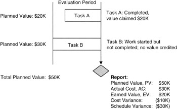
Figure 6-1: Two-Task One-Period Example.
Now in Figure 6-2, we see that we complete Task B, claim $30,000 of earned value, and calculate the variances for Period 2. Of course since there was no planned value and a big earned value, we get a positive schedule variance. Overall from the two periods combined, we get the following performance record for Tasks A and B:
PV = $50,000, EV = $50,000, AC = $60,000
Schedule variance at the end of Period 2: EV - PV = $0
Cost variance at the end of Period 2: EV - AC = -$10,000
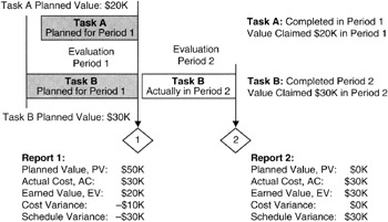
Figure 6-2: Two-Task Two-Period Example.
We are on schedule at the end of Period 2 but carry a cost variance along for the rest of the project. The project manager now begins to analyze where in the project there might be a $10,000 positive variance in another work package that could offset the cost variance from the Task A and B experience.
Three Task Example
Now as it might happen, and often does, as the work package manager is working on a pair of tasks such as we just analyzed, along comes Task C. Task C is unplanned for the current period; Task C is planned for Period 2. Nonetheless, the decision is made to work on Task A and C and let Task B go to the next period. This situation is illustrated in Figure 6-3. Only Task A is completed in Period 1. Work is started in Period 1 on Task C, but not completed; Task C will be completed in Period 2. Task B is deferred to Period 2.
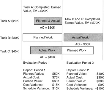
Figure 6-3: Three-Task Two-Period Example.
Penalty Costs and Opportunity Costs in Earned Value
You might have observed from the bicycle project that the value variance to the project sponsor for the one-period delay as measured in earned value is $0. By definition, the schedule variance is also $0. But in calendar terms, the project is one period late. Is it not reasonable to assign a variance to a late delivery? If the late delivery has no dollar consequence, then the late delivery has no influence on the earned value metrics. But one of the principal objectives of the earned value method is to influence project manager decision making and performance. Without consequences, the project manager will focus elsewhere. If there are dollar consequences to the late delivery, then those dollar penalties are incorporated into the period earned value or the period cost, depending on whether the dollar penalty is an opportunity cost (value) or an expensed cost (cost).
Consider this project situation: delivery of the bicycle one period late requires payment of a late delivery penalty of $500 to the ultimate customer. Such a payment is a "hard" cost expense. The $500 is expensed to the project and becomes a part of the project cost. The value of the bicycle to the sponsor remains the same, PV = $1,000. The variances now are for the whole project:
|
PV of bicycle |
= |
$1,000 |
|
AC |
= |
$1,500 = $1,000 cost + $500 penalty |
|
EV |
= |
$1,000 |
|
Cost variance |
= |
EV - AC = $1,000 - $1,500 = -$500 |
|
Schedule or value variance |
= |
EV - PV = $1,000 - $1,000 = $0 |
A late delivery also may present a depreciation of value requiring a discount to be applied to the earned value. We have studied the discount issues in prior chapters. Let us say that a one-period delay requires a 5% discount of value. No dollar penalties are involved. The 5% discount is an opportunity cost requiring an adjustment of the earned value. The bicycle project variances would then be:
|
PV |
= |
$1,000 (The performance baseline does not change) |
|
EV |
= |
(1 - 0.05) * $1,000 = $950 (Opportunity cost is applied to the EV) |
|
AC |
= |
$1,000 |
|
Cost variance |
= |
EV - AC = $950 - $1,000 = -$50 |
|
Schedule or value variance |
= |
EV - PV = $950 - $1,000 = -$50 |
In subsequent tables and paragraphs the "value variance" will be called the "schedule variance." Make note that the schedule variance is dimensioned in dollars rather than hours, days, or weeks.
Graphing Earned Value
Let's turn our attention from numbers to graphs. Sometimes the graphical depiction is very instructive and more quickly grasped than the numbers. For the moment, let us consider the project situation as depicted in Figure 6-4. The equations from Table 6-4 have been used to draw some curves. To make it simple, the curves are actually straight lines. There is no loss of generality for having straight lines for purposes of variances. However, the slope of the cumulative line at the point of evaluation affects the forecast, so just connecting some widely spaced points may create errors in the forecast.
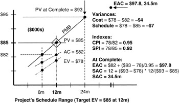
Figure 6-4: Project Example 1.
In Figure 6-4, we see a project already under way with a vertical line drawn at the evaluation point. The curves are the aggregated sums of all the work packages in the WBS up to the evaluation point. The PMB extends for the whole project. Thus, these curves represent the project situation overall. At a glance, the experienced project manager can see that the earned value curve is below the actual cost curve, so there is a cumulative unfavorable cost variance to the earned value. The earned value curve is also below the PMB, so there is a schedule variance as well.
EV curve below AC means: unfavorable cost variance
EV curve below the PMB or PV means: unfavorable schedule variance
Forecasting with Earned Value Measurements
Let us return to the bicycle now that we have a more complete set of equations to work with from Table 6-4. At the end of Period 1, we could make some forecasts:
|
Schedule performance index (SPI) |
= |
EV1/PV1 = $0/$1,000 = 0 |
|
Forecast of schedule |
= |
(PMB - EV1)/SPI = indefinite (on account of divide-by-0) |
|
Cost performance index (CPI) |
= |
EV1/AC1 = $0/(-$900) = 0 |
|
Forecast of cost |
= |
(PMB - EV1)/CPI = indefinite |
What to make of these forecasts? With no earnings, it is impossible to measure an earnings trend and therefore forecast the future from the past. What should the project manager do in such a case? With no guidance from the earned value forecast, the project manager could forecast the future or rebaseline by re-estimating the remaining work.
We can use the curves in Figure 6-4 to do some elementary forecasting. Doing so will give us a feel for the problem. Unlike the bicycle case, where the earned value was $0 and the forecast was indefinite, there are cumulative earnings for the project shown in Figure 6-4. The project manager can make a prediction by extending the cumulative earned value line until it intersects with the dollar value of the planned value at completion. At this intersection, the cumulative project earned value equals the cumulative value of the project. The extended time on the horizontal axis at the point where the cumulative earned value equals the planned value at completion is the schedule at completion.
The project manager must be careful at this point. The slope of the extension must match the slope of the cumulative earned value curve at the point of evaluation. The slope is the ratio of a small increment of the vertical scale divided by a small increment of the horizontal scale. On the figure we are working with, the horizontal scale is time, so the slope is:
ΔEV/ΔT, where Δ means "small increment of
This slope, ΔEV/ΔT, tells us we are earning value at a certain rate of so many dollars, $ΔEV, per time unit, AT. If the remaining value to be earned is PVremaining, then the time required to earn that much value is:
Remaining time = ΔT * PVremaining/ΔEV
A numerical example would probably be helpful at this point. Suppose there is $10,000 of remaining value to be earned on a project in the remaining periods. Let us say that in the last reporting period the earned value was $1,000, but that overall the earnings to date have been $24,000 over six periods. On average, the $EV/period is $24,000/6 = $4,000/period. Using this average, we could forecast that 2.5 periods remain to earn the remaining $10,000. Using our formula: 2.5 = 6 * $10,000/$24,000.
However, in the last period, earnings have slowed to $1,000/period. Thus, applying the formula to the performance as of the last period to find out how many remaining periods there are, we have: 10 = 1 * $10,000/$1,000. Which forecast is correct, 2.5 periods or 10 periods? It depends. It depends on the judgment of the project manager regarding whether or not the performance in the last period is representative of the future expectations. If the last period is not representative, then the overall average that uses much more information should be used. When working with statistics like average, in general the more information incorporated, the better is the forecast.
Estimate at Completion, Estimate to Complete
There is a simple formula that ties the EAC and ETC together:
EAC = ETC + AC to date
The actual cost to date is obtained right off the P&L. However, the ETC is somewhat problematic. There are three ways to calculate ETC:
- Apply the earned value formula: ETC = PVremaining * ACto date/EVto date
- Re-estimate the ETC and then rebaseline the remaining planned value as described elsewhere
- ETC = PVremaining
Of course, all three methods will provide a different answer. Which to use is a decision to be made by the project manager considering the situation of the project.
Time Centric Earned Value
What we have discussed to this point is the traditional and most robust form of earned value. Whenever the resources are available to apply the method, it should be done because it focuses on the accomplishments that lead to project value being delivered as promised. However, the collection and reporting of actual cost is often impractical, thereby rendering the quantitative measures unobtainable. In that event, there is an alternative, though less robust, earned value method named "time-centric earned value," [12] first described to the industry in the author's presentation [13] with James R. Sumara to the PMI National Symposium in 1997.
Time Centric Principles
The main idea behind the time-centric earned value system is to set a PMB based on planned work package starts and finishes over the course of the project. Time-centric earned value is very close to the concept of "work units" or "standard units of work" as a measure of accomplishment rather than a specific dollarized WBS cost account. Instead of a standard unit of work, however, time-centric earned value focuses on a completed task, with unknown actual cost, as the unit of value in the project.
Although a dollar value is not assigned to each work package start or finish, the total collection of starts and finishes, if executed completely, does represent the total scope (and value) of the project. The total scope of the project does have a dollar planned value (budget).
The historical reporting for purposes of determining variances remains a component of the time-centric system. Instead of earning a dollar value, what is earned is a start or a finish. The PMB is a set of planned starts and planned finishes. Therefore, there is a variance that can be defined thus:
|
Variance (start) |
= |
Earned starts - Planned starts |
|
Variance (finish) |
= |
Earned finishes - Planned finishes |
All the rules we have discussed about what constitutes a claim of credit apply. The definitions of start and finish used in the traditional method to gate the expenses for purposes of calculating the variances to the earned and planned value still apply, but apply to whether a task start can be claimed and not whether actual cost is to be applied. So too do the ideas of rebaselining, calculating the ETC, and the EAC still apply, but apply to the idea of finishing the project on a time basis and not a cost basis.
Time-centric indexes can also be defined and calculated:
|
Task start performance index (TSPI) |
= |
(Earned starts)/(Planned starts) |
|
Task finish performance index (TFPI) |
= |
(Earned finishes)/(Planned finishes) |
Figure 6-5 provides an illustration of a project wherein the PMB has 20 starts in the first three periods. We see in this figure that the project team has indeed started 20 tasks, but the starts are at a different pace than planned. We can calculate a variance for each period:
|
Start variance1 |
= |
3 - 5 = -2 starts |
|
Start variance2 |
= |
9 - 10 = -1 start |
|
Start variance3 |
= |
6 - 5 = 1 start |
|
Start variance4 |
= |
2 - 0 = 2 starts |
|
Σ (All variances) |
= |
0 start |
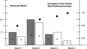
Figure 6-5: Time-Centric Project Start Example.
At the end of four periods, the project is caught up on starts. The project manager can also forecast how soon the project will attain all the starts planned in the PMB using the performance indexes. Table 6-6 provides the start performance metrics. Similarly, we see in Figure 6-6 the finish performance for the example project. Variances similar to the start variances can be calculated; indexes can also be calculated as was done for the project starts. Table 6-7 provides those calculations.
|
Planned Starts by Month [*] |
Actual Starts by Month |
Monthly Index |
Cumulative Index |
Forecasted Finish |
|---|---|---|---|---|
|
Month 1: 5 starts |
Month 1: 3 starts |
TSPI1 = 3/5 = 0.6 |
Cum Starts = 3 Remaining = 17 Cum = 3/5 = 0.6 |
Adjusted remaining starts = 17/0.6 = 28 Forecast schedule remaining = 2 months * 28/17 = 3.3 months |
|
Month 2: 10 starts |
Month 2: 9 starts |
TSPI2 = 9/10 = 0.9 |
Cum Starts = 12 Remaining = 8 Cum = 12/15 = 0.8 |
Adjusted remaining starts = 8/0.8 = 10 Forecast schedule remaining = 1 month * 10/8 = 1.25 months |
|
Month 3: 5 starts |
Month 3: 6 starts |
TSPI3 = 6/5 = 1.2 |
Cum Starts = 18 Remaining = 2 Cum = 18/20 = 0.9 |
Adjusted remaining starts = 2/0.9 = 2.2 Forecast schedule remaining = 0 months * 2.2/2 = 0 months (no remaining schedule available) |
|
Month 4: 0 starts |
Month 4: 2 starts |
TSPI4 = 2/0 = indefinite |
Cum Starts = 20 Remaining = 0 Cum = 20/20 = 1.0 |
Adjusted remaining starts = 0/1 = 0 Forecast schedule remaining = 0/0 = indefinite |
|
[*]See related figure for a graphical presentation of this example. |
||||
|
Planned Finishes by Month [*] |
Actual Finishes by Month |
Monthly Index |
Cumulative Index |
Forecasted Finish |
|---|---|---|---|---|
|
Month 4: 3 finishes |
Month 1: 3 finishes |
TFPI1 = 3/3 = 1 |
Cum Finishes = 3 Remaining = 17 Cum = 3/3 = 1.0 |
Adjusted remaining finishes = 17/1 = 17 Forecast schedule remaining = 2 months * 17/17 = 2 months |
|
Month 5: 10 finishes |
Month 2: 7 finishes |
TFPI2 = 7/10 = 0.7 |
Cum Finishes = 10 Remaining = 10 Cum = 10/13 = 0.77 |
Adjusted remaining finishes = 10/0.77 = 10.4 Forecast schedule remaining = 1 month * 10.4/10 = 1.04 months |
|
Month 6: 7 finishes |
Month 3: 6 finishes |
TFPI3 = 6/7 = 0.86 |
Cum Finishes = 16 Remaining = 4 Cum = 16/20 = 0.8 |
Adjusted remaining finishes = 4/0.8 = 5 Forecast schedule remaining = 0 months * 5/4 = 0 months (no remaining schedule available) |
|
Month 7: 0 finishes |
Month 4: 4 finishes |
TFPI4 = 4/0 = indefinite |
Cum Finishes = 20 Remaining = 0 Cum = 20/20 = 1.0 |
Adjusted remaining finishes = 0/1 = 0 Forecast schedule remaining = 0/0 = indefinite |
|
[*]See related figure for a graphical presentation of this example. |
||||
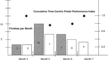
Figure 6-6: Time-Centric Project Finish Example.
Forecasting with the Time Centric System
Just like in the traditional earned value system, forecasts can be made using the same formula as we developed for the forecast in that system:
- Forecast = Actual performance + Remaining performance/Index
For example, in the first period the actual starts are 3, the remaining performance for the project is 17, and the index is 0.6. The forecast is therefore:
|
First period index |
= |
3/5 = 0.6 |
|
Actual starts |
= |
3 |
|
Forecast |
= |
3 + 17/0.6 = 3 + 28.3 = 31.3 starts |
where 31.3 = "equivalent" starts.
How should the project manager interpret the forecast given above? The equivalent starts represent the length of the project as though the PMB were 31.3 starts rather than 20. In other words, based on the performance in the first period, the project is forecasted to be 11.3/20 = 56.5% longer in schedule than the PMB. Fortunately, by the second period the trend line turns more favorable:
|
Cumulative index |
= |
12/15 = 0.8 |
|
Cumulative starts |
= |
12 |
|
Forecast |
= |
12 + 8/0.8 = 22 starts |
where 22 = "equivalent" starts.
As with the traditional earned value system, the most valuable contribution of the calculations is to stimulate the project team to take action necessary to deliver the value to the project sponsor as defined on the project balance sheet and specified in the project charter. Whether or not the time-centric or traditional system is used, the calculations should have the same effect and provide the requisite catalyst to correct whatever is not working well in the project.
[12]The original work on "time-centric earned value" was done by the author and colleague James Sumara while working with the Lanier Worldwide business unit of Harris Corporation in the mid-1990s. Although the traditional earned value system was well known and practiced at Harris, the Lanier Worldwide business unit did not have the mechanisms for complete collection of the actual cost of the labor employed for internal projects. Time-centric earned value was developed for the Lanier Worldwide project office to fill the need for an earned value reporting tool.
[13]Goodpasture, John C. and Sumara, James R., Earned Value — The Next Generation — A Practical Application for Commercial Projects, PMI '97 Seminars and Symposium Proceedings, Project Management Institute, Newtown Square, PA, 1997.
Summary of Important Points
Table 6-8 provides the highlights of this chapter.
|
Point of Discussion |
Summary of Ideas Presented |
|---|---|
|
The expense (P&L) statement |
|
|
Lean thinking |
|
|
Managing with three-point estimates |
|
|
Earned value concept |
|
|
Dollar-sizing the cost accounts |
|
|
Time-centric earned value |
|
References
1. Womack, James P. and Jones, Daniel T., Lean Thinking, Simon & Schuster, New York, 1996, Introduction, pp. 15–28.
2. Fleming, Quentin W. and Koppelman, Joel M., Earned Value Project Management, Second Edition, Project Management Institute, Newtown Square, PA, 2000, chap. 3, pp. 25–33.
3. Under Secretary of Defense (Acquisition), DoDI 5000.1 The Defense Acquisition System, Department of Defense, Washington, D.C., 1989; and its predecessor instruction: DoD Comptroller, DoDI 7000.2 Performance Measurement for Selected Acquisitions, Department of Defense, Washington, D.C., 1967.
4. Kemps, Robert R., Project Management Measurement, Humphrey's and Associates, Inc., Mission Viejo, CA, 1992, chap. 16, pp. 97–107.
5. Fleming, Quentin W. and Koppelman, Joel M., Appendix I, pp. 157–181 and Appendix II, pp. 183–188.
6. Goodpasture, John C. and Sumara, James R., Earned Value — The Next Generation — A Practical Application for Commercial Projects, PMI '97 Seminars and Symposium Proceedings, Project Management Institute, Newtown Square, PA, 1997.
Preface
- Project Value: The Source of all Quantitative Measures
- Introduction to Probability and Statistics for Projects
- Organizing and Estimating the Work
- Making Quantitative Decisions
- Risk-Adjusted Financial Management
- Expense Accounting and Earned Value
- Quantitative Time Management
- Special Topics in Quantitative Management
- Quantitative Methods in Project Contracts
EAN: 2147483647
Pages: 97
