Organizing and Estimating the Work
Overview
There likely is no factor that would contribute more to the success of any project than having a good and complete definition of the project's scope of work.
Quentin Fleming and Joel Koppelman
Earned Value Project Management
In the normal course of project events, business leaders develop the need for a project after recognizing opportunity that can be transformed into business value. Such a project is defined on the business side of the project balance sheet. Although the business and the project team may have differences about resources and schedule, the common conveyance of ideas across the project balance sheet is scope. Understand the scope clearly and the project management team should be able to then estimate required resources, schedule, and quality. Defining scope and estimating the work are inextricably tightly coupled.
The Department of Defense, certainly a proponent of rigorous project management, sees the benefit of having a structured approach to organizing the project scope when it says that such a structure: [1]
- "Separates (an)...item into its component parts, making the relationships of the parts clear and the relationship of the tasks to be completed — to each other and to the end product — clear.
- Significantly affects planning and the assignment of management and technical responsibilities.
- Assists in tracking the status of...(project) efforts, resource allocations, cost estimates, expenditures, and cost and technical performance."
- Helps ensure that contractors are not unnecessarily constrained in meeting item requirements.
[1]Editor, MIL-HDBK-881, OUSD(A&T)API/PM, U.S. Department of Defense, Washington, D.C., 1998, paragraph 1.4.2.
Organizing the Scope of Work
Organizing and defining the project scope of work seems a natural enough step and a required prerequisite to all analytical estimates concerning projects. Though constructing the logical relationships among the deliverables of the project scope appears straightforward, in point of fact developing the scope structure is often more vexing than first imagined because two purposes are to be served at the same time: (1) provide a capture vessel for all the scope of the project and (2) provide quantitative data for analysis and reporting to project managers and sponsors.
Work Definition and Scoping Process
The general process (input, methods, output) for scope or work definition and organization is given in Figure 3-1. Inputs to the process are assembled from all the ideas and prerequisite information from the business side of the project balance sheet that describe the desired outcomes of the project, including constraints, assumptions, and external dependencies. Methods are the steps employed in the scope definition process to organize this information, decompose the given material into a finer granularity of functional and technical scope, and relate various elements of the project deliverables to each other. The outcome of the work definition and scoping process is an "organization of the deliverables" of the project, often in hierarchical list or chart form, or in relational form that supports multiple views.
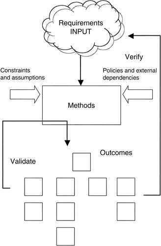
Figure 3-1: Work Definition and Scoping Process.
We should note that the "organization of the deliverables" is not an organization chart of the project in the sense of responsibility assignments, reporting, and administration among project members. The "organization" we speak of is the logical relationship among, and definition of, the deliverables for which the project manager makes quantitative estimates for resources needs, risks, and schedule requirements on the project side of the project balance sheet. The name given to the organization of project deliverables is work breakdown structure (WBS). Suffice to say: all the scope of the project is contained in the WBS.
The process includes loops to validate and verify the completeness of the WBS. Validation refers to determining that everything on the WBS is there for a reason and is not inappropriate to the project scope. Validation also determines the proper hierarchical level for all deliverables and ensures hierarchical integrity. Verification is closely aligned with validation. Verification extends the concept back to the business owner or project sponsor to ensure that all scope has been accounted for and is on the WBS.
Multiple Views in Scope Organization
One purpose of the WBS organization is to serve the informational needs of those who will use the WBS in the course of managing and overseeing the project. Thus, the WBS should be organized to most effectively serve the management team. There are many possible ways to organize the information provided by the business, project team, project vendors, and others. Consider, for instance, these possibilities as illustrated in Figure 3-2: [2]
- Deliverables view: Because there are many points of view regarding project scope, more than one version of the WBS of the same project is possible as shown in Table 3-1. The preferred view is that of product or deliverables, focusing the WBS on the accomplishments of the project insofar as the sponsor or business is concerned. Unless otherwise noted, in this book the product or deliverable view will always be the view under discussion.
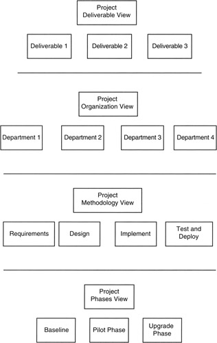
Figure 3-2: Project Views on the WBS.Table 3-1: Views of the Project Scope View
Scope Organization
Business owner or project sponsor
Organize by deliverables to the business required to make good on the business case
Business financial manager
Organize by types or uses of money, such as R&D funds, capital funds, expense funds, O&M funds
Project manager
Organize by methodological steps, such as design, develop, test and evaluation, training, and rollout
Project developer
Organize by phases such as the baseline phase, upgrade phase, pilot phase, production phase
Manufacturing, operations, and maintenance provider
Organize by life cycle steps, such as plan, implement, manufacture, rollout, maintain
Customer or user
Organize by deliverables to the user, such as the training and operational deliverables only available to the user
- Organizational view: Some project scopes are organized according to the departments that will deliver the work. Organizational project scope may be appropriate if there are facility, technology, or vendor boundaries that must be factored into the scope structure. For instance, in the semiconductor industry, there are usually quite significant boundaries between design, wafer fabrication, and end-device assembly and test.
- Methodology view: The methodology used to execute the project often influences scope, either temporally or in terms of scope content. Projects in different domains, for instance software development, building construction, and new consumer products, generally follow differing methodologies from planning to rollout and project completion, thereby generating many different deliverables along the way. These deliverables are often organized into methodology phases, or builds, on the WBS.
- Phases view: Scope phases that respond to the business needs or business capacity add a temporal dimension to the WBS organization. Ordinarily, the WBS is blind to time. In fact, a useful way to think of the WBS is that the WBS is the schedule collapsed to present time; in effect, the WBS is the "present value" of the schedule. Of course, the corollary is that the schedule is merely the WBS laid out on a calendar.
The Work Breakdown Structure
The WBS has been a fixture of project management for many years. [3] The WBS is simply the organizing structure of the entire scope of the project. There is one organizing rule that governs overall: if an item is on the WBS, then that item is within the scope of the project; if an item is not on the WBS, then that item is out of scope of the project. The WBS identifies the deliverables and activities that are within the scope of the project.
The WBS is most typically shown as an ordered hierarchical list, or equivalent chart or diagram, of project deliverables. By their nature, hierarchies have levels. A higher level is an abstract of all the levels below it and connected to it. For emphasis, let us term this concept the "completeness rule" for WBSs: to wit, an element at a higher level is defined by all of, but only all of, the lower level elements that connect to it. For example, "bicycle" is an abstract of lower level items such as frame, handlebar, seat, wheels, etc. all related to and connected to "bicycle," but on the other hand "bicycle" consists of only lower level items such as frame, handlebar, seat, wheels, etc. all related to and connected to "bicycle."
At the highest level of the WBS is simply "Project," an abstract of everything in the project. Typically, "Project" is called level 1. At the next level is the first identification of distinct deliverables, and subsequent levels reveal even more detail. The next level is called level 2. Of course alpha characters could also be used, or alpha and numeric characters could be combined to distinctly identify levels and elements of the WBS. A couple of schemes are given in Figure 3-3.
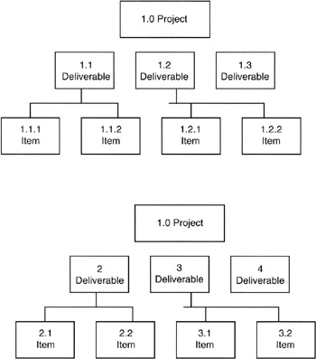
Figure 3-3: WBS Numbering Schemes.
Deliverables are typically tangible, measurable, or otherwise recognizable results of project activity. In short, deliverables are the project "nouns." The project nouns are what are left when the project is complete and the team has gone on to other things. Of course, materiel items that make up an item, like nuts and bolts, are typically not identified as deliverables themselves. Following this line of thinking, project activities (for example, design, construction, coding, painting, assembling, and so forth) are transitory and not themselves deliverables. However, the project activities required to obtain the deliverables are identified and organized by the scoping process. Activities are the actions of the project process; activities are the project "verbs. " The syntax of the WBS is then straightforward: associate with the "nouns" the necessary "verbs" required to satisfy the project scope.
Apart from showing major phases or rolling waves, the WBS is blind to time. [5] In fact, a useful way to think of the WBS is that it is the deliverables on the schedule all viewed in present time. It follows that all nouns and verbs on the WBS must be found in the project schedule, arranged in the same hierarchy, but with all the time-dependent durations and dependencies shown.
Work Breakdown Structure Standards
There are standards that describe the WBS. [6] Perhaps the most well known is the Department of Defense handbook, "MIL-HDBK-881." [8] As defined therein (with emphasis from the original), the WBS is:
- "A product-oriented family tree composed of hardware, software, services, data, and facilities. The family tree results from...efforts during the acquisition of a...materiel item.
- A WBS displays and defines the product, or products, to be developed and/or produced. It relates the elements of work to be accomplished to each other and to the end product.
- A WBS can be expressed down to any level of interest. However (if)...items identified are high cost or high risk...(then)...is it important to take the work breakdown structure to a lower level of definition."
As a standard, MIL-HDBK-881 makes definitive statements about certain "do's and don'ts" that make the WBS more useful to managers. Table 3-2 summarizes the advice from MIL-HDBK-881.
|
Scope Organization |
|---|
|
Do not include elements that are not products. A signal processor, for example, is clearly a product, as are mock-ups and Computer Software Configuration Items (CSCIs). On the other hand, things like design engineering, requirements analysis, test engineering, aluminum stock, and direct costs are not products. Design engineering, test engineering, and requirements analysis are all engineering functional efforts; aluminum is a material resource; and direct cost is an accounting classification. Thus, none of these elements are appropriate WBS elements. |
|
Program phases (e.g., design, development, production, and types of funds, or research, development, test, and evaluation) are inappropriate as elements in a WBS. |
|
Rework, retesting, and refurbishing are not separate elements in a WBS. They should be treated as part of the appropriate WBS element affected. |
|
Nonrecurring and recurring classifications are not WBS elements. The reporting requirements of the CCDR will segregate each element into its recurring and nonrecurring parts. |
|
Cost-saving efforts such as total quality management initiatives, should-cost estimates, and warranty are not part of the WBS. These efforts should be included in the cost of the item they affect, not captured separately. |
|
Do not use the structure of the program office or the contractor's organization as the basis of a WBS. |
|
Do not treat costs for meetings, travel, computer support, etc. as separate WBS elements. They are to be included with the WBS elements with which they are associated. |
|
Use actual system names and nomenclature. Generic terms are inappropriate in a WBS. The WBS elements should clearly indicate the character of the product to avoid semantic confusion. For example, if the Level 1 system is Fire Control, then the Level 2 item (prime mission product) is Fire Control Radar. |
|
Treat tooling as a functional cost, not a WBS element. Tooling (e.g., special test equipment and factory support equipment like assembly tools, dies, jigs, fixtures, master forms, and handling equipment) should be included in the cost of the equipment being produced. If the tooling cannot be assigned to an identified subsystem or component, it should be included in the cost of integration, assembly, test, and checkout. |
|
Include software costs in the cost of the equipment. For example, when a software development facility is created to support the development of software, the effort associated with this element is considered part of the CSCI it supports or, if more than one CSCI is involved, the software effort should be included under integration, assembly, test, and checkout. Software developed to reside on specific equipment must be identified as a subset of that equipment. |
|
Do's and don'ts are excerpted from MIL-HDBK-881. |
Adding Organizational Breakdown Structure and Resource Assignment Matrix to the Work Breakdown Structure
In fact, the WBS is not one entity, but actually three:
- The WBS itself is the hierarchical structure of deliverables (nouns), and when applying the WBS in the context of contractor-subcontractor, the prime WBS is often referred to as the project or program WBS (PWBS) and the subcontractor's WBS is referred to as the contract or contractor WBS (CWBS).
- A structure similar to the WBS can be made for the organizations that participate in the project. Such a structure is called the organizational breakdown structure (OBS).
- The OBS and the WBS are cross-referenced with the resource assignment matrix (RAM).
Figure 3-4 shows the three component parts working together.
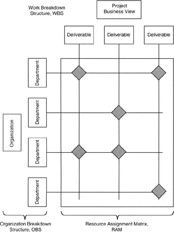
Figure 3-4: WBS Components.
The RAM is where the analytical aspects of the WBS come into play. At each node of the RAM where there is an intersection of the OBS and WBS, the resource commitment of the organizations is allocated to the WBS. From the RAM, the resources can be added vertically into the WBS hierarchy and horizontally into the OBS hierarchy. Such an addition is shown in Figure 3-5. Note that the following equation holds:
∑ (All WBS resources) = ∑ (All OBS resources) = Project resources
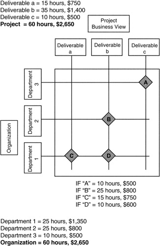
Figure 3-5: Adding Up the RAM.
Budgeting with the Work Breakdown Structure
From Figure 3-5, we see that OBS department budgets and WBS project budgets intersect. Eventually, these budgeted items must find their way to the chart of accounts of the business. Let us introduce additional nomenclature to go with the chart of accounts:
- The WBS itself is often numbered hierarchically for each work element identified. The WBS numbering scheme is sometimes called the "code of accounts." [9]
- At the lowest level of the WBS where cost is assigned, the WBS element is called a "work package." The project manager assigns responsibility to someone on the project team for the work package.
- Work packages need not all be at the same level on the WBS. However, to make the WBS uniform in level for data collection and reporting, "pull downs" of "dummy" levels are employed. As an example, let us say that "bicycle" is decomposed down to level 3 with work packages 1.1.1 (stationary parts) and 1.1.2 (moving parts). Let us say that there is also a "wagon" on the WBS, and that "wagon" ends at level 4 with work package 1.2.1.1 (wheels) and 1.2.1.2 (axles). To create uniform metric reporting at the fourth level of the WBS we would create a "level 4 pull down" of "bicycle" with dummy elements 1.1.1.1 (stationary parts) and 1.1.2.1 (moving parts) that have the exact same content as their third-level parents. Similarly, there would be a fourth-level pull down for "wagon" for element 1.2.2. Our example WBS is illustrated in Figure 3-6.
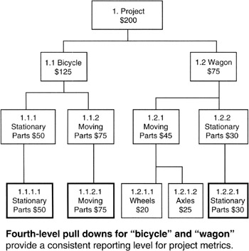
Figure 3-6: Bicycle and Wagon. - Cost accounts are roll ups of work packages and any in-between levels of the WBS. The project manager assigns responsibility for performance of a cost account to someone on the team, and, by extension, that person is responsible for the work packages that roll into the cost account.
Cost Accounts and Work Packages
Returning to Figure 3-5, we see that there are four work packages: A, B, C, and D. What, then, are the cost accounts? Typically, cost accounts are either one or more work packages rolled up vertically (project view) or horizontally (organizational view). Depending on the project management approach regarding "matrix management" and project responsibilities, either roll up could be possible. [10] So, there are either three cost accounts corresponding to "depart- ments 1, 2, and 3" or three cost accounts corresponding to "deliverables a, b, and c." We know from prior discussion that the total project expense is not dependent on whether the cost accounts are rolled up vertically or horizontally. Therefore, the choice is left to the business to decide how responsibility is to be assigned for project performance.
Now, let us consider the chart of accounts of the business. The chart might well be shown as in Figure 3-7. We see that Organization has expense and Project has expense. We would not want to count expenses in both categories since that would be counting the same expense twice. If both were fed to the chart of accounts, an accounting process known as "expense elimination" would be required to reconcile the total expenses reported. To avoid the accounting overhead to eliminate redundant expenses, the solution, of course, is not to connect one or the other roll up to the chart of accounts. That is, if the project is going to have an account on the chart of accounts, then the project expenses would not roll up under department and organization; instead, project-specific, or direct, expenses would roll up under the project itself.
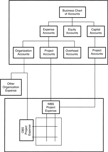
Figure 3-7: Chart of Accounts and the WBS.
We see also on the chart of accounts a place for capital accounts. From Chapter 1, we know that capital accounts represent asset values that have not yet been "expensed" into the business expense accounts. Capital purchases made on behalf of projects are usually not recorded as project expenditures at the time the purchases are made. Rather, the practice is to depreciate the capital expenditure over time and assign to the project only the depreciation expense as depreciation is recorded as an expense in the chart of accounts. As capital is depreciated from the capital accounts, depreciation becomes expense in the expense accounts, flowing downward through the WBS to the RAM where depreciation expense is assigned to a work package.
In the foregoing discussion we established an important idea: the WBS is an extension of the chart of accounts. Just as a WBS element can describe a small scope of work, so also can a WBS element account for a small element of cost or resource consumption (hours, facilities usage, etc.).
Of course, not only is the budget distributed among the work packages on the RAM, but so also are the actual performance figures gathered and measured during project execution. Thus, work package actuals can be added across the OBS and up the WBS hierarchy all the way to the level 1 of the WBS or Organization of the OBS. The variance to budget is also additive across and up the WBS. In subsequent chapters, we will discuss earned value as a performance measurement and forecasting methodology. Within the earned value methodology is a concept of performance indexes, said indexes computed as ratios of important performance metrics. Indexes per se are not additive across and up the WBS. Indexes must be recomputed from summary data at each summarization level of the WBS or the OBS.
Work Breakdown Structure Dictionary
We add to our discussion of the WBS with a word about the WBS dictionary. It is common practice to define the scope content, in effect the statement of work, for each element of the WBS in a WBS dictionary. We see that this is an obvious prerequisite to estimating any specific element of the WBS. Typically, the WBS dictionary is not unlike any written dictionary. A dictionary entry is a narrative of some form that is explanatory of the work that needs to be done and the expected deliverable of the work package. For all practical purposes, the dictionary narrative is a scope statement for the "mini-project" we call the work package.
The total scope assigned to a cost account manager is then defined as the sum of the scope of each of the related work packages defined in the WBS dictionary. Though cost, facility requirements, skills, hours, and vendor items are not traditionally contained or defined in the dictionary, the total resources available to the cost account manager for the scope in the WBS dictionary are those resources assigned to each of the constituent work packages.
Work Breakdown Structure Baseline
For quantitative estimating purposes, we need a target to shoot at. It is better that the target be a static target, not moving during the time of estimation. The scope captured on the WBS at the time estimating begins is the project "baseline scope." Baselines are "fixed" until they are changed. Changing the baseline is a whole subject unto itself. Suffice to say that once resources are assigned to a baseline, and then that baseline is changed, the task of the project manager and project administrator is to map from the RAM in the baseline to the RAM of the changed baseline. A common practice is to consider all resource consumption from initial baseline to the point of rebaseline to be "sunk cost," or actuals to date (ATD), not requiring mapping. Expenditures going forward are either mapped from the initial baseline, or the WBS of the subsequent baseline is re-estimated as "estimate to complete" (ETC). Total project cost at completion then becomes:
Cost at completion = ATD of WBS Baseline-1 + ETC of WBS Baseline-2
The practical effect of rebaselining is to reset variances and budgets on the WBS. The WBS dictionary may also be modified for the new baseline. Considering the need for cost and performance history, and the connection to the chart of accounts, there are a couple of approaches that can be taken. To preserve history, particularly valuable for future and subsequent estimations, WBS Baseline-1 may be given a different project account number on the chart of accounts from that assigned to the WBS Baseline-2. The cost history of WBS Baseline-1 and the WBS Baseline-1 dictionary can then be saved for future reference.
A second and less desirable approach from the viewpoint of preserving history is to make a lump sum entry into the chart of accounts for the ATD of WBS Baseline-1. Then WBS Baseline-2 is connected to the chart of accounts in substitution for WBS Baseline-1 and work begins anew.
[2]There is no single "right way" for constructing a WBS of a given project, though there may be policies and standard practices in specific organizations or industries that govern the WBS applied therein. The only rule that must be honored is that all the project scope must appear on the WBS.
[3]A brief but informative history of the development of the WBS, starting as an adjunct to the earliest development of the PERT (Program Evaluation Review Technique) planning and scheduling methodology in the late 1950s in the Navy, and then finding formalization in the Department of Defense in 1968 as MIL-STD-881, subsequently updated to MIL-HDBK-881 in 1998, can be found in Gregory Haugan's book, Effective Work Breakdown Structures. [4]
[3]Haugan, Gregory T., Effective Work Breakdown Structures, Management Concepts, Vienna, VA, 2001, chap. 1, pp. 7–13.
[5]Rolling waves is a planning concept that we discuss more in subsequent chapters. In short, the idea is to plan near-term activities in detail, and defer detailed planning of far-future activities until their time frame is more near term.
[6]The WBS is covered extensively in publications of the Department of Defense (MIL-HDBK-881) and the National Aeronautics and Space Administration (Work Breakdown Structure Guide, Program/Project Management Series, 1994) as well as A Guide to the Project Management Body of Knowledge, [7] among others.
[6]A Guide to the Project Management Body of Knowledge (PMBOK Guide) — 2000 Edition, Project Management Institute, Newtown Square, PA, chap. 5.
[8]Editor, MIL-HDBK-881, OUSD(A&T)API/PM, U.S. Department of Defense, Washington, D.C., 1998, paragraph 1.6.3.
[9]A Guide to the Project Management Body of Knowledge (PMBOK Guide) — 2000 Edition, Project Management Institute, Newtown Square, PA, chap. 2.
[10]See A Guide to the Project Management Body of Knowledge [11] for a discussion of project management organizing ideas and matrix management. For a strongly "projectized" approach, the cost accounts will be in the project view, summed vertically, with "project" managers assigned. For an organizational approach to the project, the cost accounts will be in the organizational view, summed horizontally, with an "organizational" manager assigned.
[10]A Guide to the Project Management Body of Knowledge (PMBOK Guide) — 2000 Edition, Project Management Institute, Newtown Square, PA, chap. 2.
Estimating Methods for Projects
There is no single method that applies to all projects. Estimating is very domain specific. Construction, software, pharmaceuticals, packaging, and services, just to name a few of perhaps hundreds if not thousands of domains, have unique and specific estimating methodologies. Our intent is to discuss general principles that apply universally. Project managers are in the best position to adapt generalities to the specific project instance.
Estimating Concepts
The objectives of performing an estimate are twofold: to arrive at an expected value for the item being estimated and to be able to convey a figure of merit for that estimate. In this book we will focus on estimating deliverables on a WBS. The figure of merit we will use is the confidence interval that is calculable from the statistical data of the underlying distribution of the expected value of the estimate.
Most estimating fits into one of four models as illustrated in Figure 3-8:
- Top-down value judgments from the business side of the project balance sheet conveyed to the project team
- Similar-to judgments from either side of the project balance sheet, but most often from the business side
- Bottom-up facts-driven estimates of actual work effort from the project side of the project balance sheet conveyed to the project sponsor
- Parametric calculations from a cost-history model, developed by the project team, and conveyed to the project sponsor
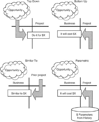
Figure 3-8: Estimating Concepts.
Naturally, it is rare that a project would depend only on one estimating technique; therefore, it is not unusual that any specific project team will use all the estimating methods available to it that fit the project context. However, let us consider them one by one.
Top-Down Estimates
Top-down estimates could be made by anyone associated with the project, but most often top-down estimates come from the business and reflect a value judgment based on experience, marketing information, benchmarking data, consulting information, and other extra-project information. Top-down estimates rarely have concrete and verifiable facts of the type needed by the project team to validate the estimate with the scope laid out on the WBS.
Working with top-down estimates requires the steps shown in Table 3-3. Project risks are greatest in this estimating methodology, and overall cost estimates are usually lowest. In its purest form, top-down estimating foregoes the quantitative information that could be developed by the project team regarding the project cost. Usually, if there is an independent input to cost developed by the project team, the purpose of such an independent input from the project side is to provide comparative data with the top-down estimate. Such a comparison serves to establish the range or magnitude of the risks of being able to execute the project for the top-down budget. Because risks are greatest in top-down estimating, the risks developed in response to top-down budgets require careful identification, minimization planning, and estimation before the project begins. Risks are quantified and made visible on the project side of the project balance sheet.
|
Step |
Description |
|---|---|
|
Receive estimates from the business |
Estimates from the business reflect a judgment on the investment available given the intended scope and value to the business. |
|
Interview business leaders to determine the intended scope |
Scope is the common understanding between the business and the project. Interviews provide the opportunity to exchange information vital to project success. |
|
Verify assumptions and validate sources, if any |
The business judgment on investment and value is based on certain assumptions of the business managers and may also include collateral information that is useful to the project manager. |
|
Develop WBS from scope |
WBS must contain all the scope, but only the scope required by the business sponsors. |
|
Allocate top-down resources to WBS |
Allocation is a means of distributing the investment made possible by the business to the elements of scope on the WBS. |
|
Cost account managers identify risks and gaps |
Cost account managers have responsibility for elements of the WBS. They must assess the risk of performance based on the allocation of investment to the WBS made by the project manager. |
|
Negotiate to minimize risks and gaps |
Once the risks are quantified and understood, a confidence estimate can be made of the probability of meeting the project scope for the available investment. Negotiations with the business sponsors narrow the gap between investment and expected cost. |
|
Top-down estimate to the business side of project balance sheet |
The business makes the judgment on how much investment to make. This investment goes on the business side of the project balance sheet. |
|
Expected value estimate and risks to project side of balance sheet |
Once the allocation is made to the WBS, there is opportunity for the project manager to develop the risks to performance, the expected value, and the confidence of meeting the sponsor's objectives. |
A common application of the top-down methodology is in competitive bidding to win a project opportunity as a contractor to the project sponsor. In this scenario, the top-down estimate usually comes from a marketing or sales assessment of what the market will bear, what the competition is bidding, and in effect "what it will take to win." If the top-down estimate is the figure offered to the customer as the price, then the project manager is left with the task of estimating the risk of performance and developing the risk management plan to contain performance cost within the offered price:
Top-down offer to do business = Independently estimated cost of performance offered + Risk to close gap with top-down offer
From the steps in Table 3-3, we see that the project manager must allocate the top-down budget to the WBS. Doing so involves the following quantitative steps:
- Develop the WBS from the scope statement, disregarding cost.
- By judgment, experience, prototyping, or other means, determine or identify the deliverable of least likely cost, or the deliverable that represents the smallest "standard unit of work." Give that deliverable a numerical cost weight of 1 and call it the "baseline" deliverable, B. This procedure normalizes all costs in the WBS to the cost of the least costly deliverable.
- Estimate the normalized cost of all other deliverables, D, as multiples, M, of the baseline deliverable: Di = Mi * B, where M is a random variable with unknown distribution and "i" has values from 1 to n. "n" is the number of deliverables in the WBS.
- Sum all deliverable weights and divide the sum into the available funds to determine an absolute baseline cost of the least costly deliverable.
($Top-down budget)/(∑Mi) = Allocated cost of baseline task B
- A "sanity check" on the cost of B is now needed. Independently estimate the cost of B to determine an offset, plus or minus, between the allocated cost and the independent estimate. This offset, O, is a bias to be applied to each deliverable in the WBS. The total bias in the WBS is given by:
Total cost bias in WBS = n * O
- Complete the allocation of all top-down budgets to the deliverables in the WBS according to their weights.
- It is helpful at this point to simplify the disparate deliverables on the WBS to an average deliverable and its statistics. We know from the Central Limit Theorem that the average deliverable will be Normal distributed, so the attributes of the Normal distribution will be helpful to the project manager:
Average deliverable cost = αd = (1/n) * ∑ [Di + (Mi * O)]
σ2 of average deliverable = (1/n) * ∑[(Di + O) - αd]2, and
σ of average deliverable = √(1/n) * ∑[(Di + O) - αd]2
It is easier to calculate these figures than it probably appears from looking at the formulas. Table 3-4 provides a numerical example. In this example, a $30,000 top-down budget is applied to a WBS of seven deliverables. An offset is estimated at 23% of the allocated cost. Immediately, it appears that there may be a $6,900 risk to manage (23% of $30,000). However, we see from the calculations employing the Normal distribution that the confidence of hitting the top-down budget is only 24%, and with the $6,900 risk included, the confidence increases to only 50%. At 68% confidence, the level needed for many firms to do fixed price bidding, the risk increases significantly. Clearly if the risk is to be reduced, then the scope will have to be downsized or the budget increased, or more time given to estimating the offsets in order for this project to go forward.
|
WBS Element |
Weight, Mi |
Allocated Budget, Di |
Allocated Budget + (Mi * O) |
Distance2 (d - average d)2 |
|---|---|---|---|---|
|
a |
b |
c |
d |
e |
|
1 |
||||
|
1.1.1 |
8 |
$10,435 |
$12,835 |
57,204,324 |
|
1.1.2 |
5 |
$6,522 |
$8,022 |
7,564,208 |
|
1.1.3 |
1 |
$1,304 |
$1,604 |
13,447,481 |
|
1.2.1 |
2 |
$2,609 |
$3,209 |
4,254,867 |
|
1.2.2 |
2.5 |
$3,260 |
$4,010 |
1,591,202 |
|
1.3.1 |
1.5 |
$1,957 |
$2,407 |
8,207,691 |
|
1.3.2 |
3 |
$3,913 |
$4,813 |
210,117 |
|
Totals: |
23 |
$30,000 |
$36,900 |
92,479,890 |
|
Given: Top-down budget = $30,000 Evaluated least costly baseline deliverable, B = $1,304.35 Estimated independent cost of B = $1,604.35 Calculated baseline offset, O, = $300 = $1,604.35 - $1,304.35 |
||||
|
n = 7 ∑ Mi = 23 ∑ Di = ∑(Mi * B) = $30,000 Average deliverable, average d, with offset = $36,900/7 = $5,271 Variance, σ2 = 92,479,890/7 = 13,211,413 Standard deviation, σ = $3,635 |
||||
|
Confidence calculations: Total standard deviation of WBS = √7* σ2 = √92,479,890 = $9,616 24% confidence: WBS total ≤ $30,000 [*] 50% confidence: WBS total ≤ $36,900 68% confidence: WBS total ≤ $36,900 + $9,616 = $46,516 |
||||
|
[*]From lookup on single-tail standard Normal table for probability of outcome = ($36,900 -$30,000)/$9,616 = 0.71σ below the mean value. Assumes summation of WBS is approximately Normal with mean = $36,900 and a = $9,616. |
||||
Once the risks are calculated, all the computed figures can be moved to the right side of the project balance sheet. Let us recap what we have so far. On the business side of the project balance sheet, we have the top-down budget from the project sponsors. This is a value judgment about the amount of investment that can be afforded for the deliverables desired. On the right side of the balance sheet, the project manager has the following variables:
- The estimated "fixed" bias between the cost to perform and the available budget. In the example, the bias is $6,900.
- The average WBS for this project and the statistical standard deviation of the average WBS. In this example, the average WBS is $36,900 (equal to the budget + bias) and the standard deviation is $9,616.
- And, of course, the available budget, $30,000.
As was done in the example, confidences are calculated and the overall confidence of the project is negotiated with the project sponsor until the project risks are within the risk tolerance of the business.
Similar-To Estimates
"Similar-to" estimates have many of the features of the top-down estimate except that there is a model or previous project with similar characteristics and a cost history to guide estimating. However, the starting point is the same. The business declares the new project "similar to" another completed project and provides the budget to the new project team based on the cost history of the completed project. Of course, some adjustments are often needed to correct for the escalation of labor and material costs from an earlier time frame to the present, and there may be a need to adjust for scope difference. In most cases, the "similar-to" estimate is very much like a top-down estimate except that there is usually cost history at the WBS deliverable level available to the project manager that can be used by the project estimating team to narrow the offsets. In this manner, the offsets are not uniformly proportional as they were in the top-down model, but rather they are adjusted for each deliverable to the extent that relevant cost history is available.
The quantitative methods applied to the WBS are not really any different from those we employed in the top-down case except for the individual treatment of the offsets. Table 3-5 provides an example. We assume cost history can improve the offset estimates (or provide the business with a more realistic figure to start with). If so, the confidence in budget developed by the business as a "similar to" is generally much higher.
|
WBS Element |
Allocated Budget from Cost History, Di |
Offset |
Allocated Budget + (Mi * O) |
Distance2 (d - average d)2 |
|---|---|---|---|---|
|
a |
b |
c |
d |
e |
|
1 |
||||
|
1.1.1 |
$10,435 |
$200 |
$10,635 |
39,813,357 |
|
1.1.2 |
$6,522 |
-$100 |
$6,422 |
4,396,315 |
|
1.1.3 |
$1,304 |
$300 |
$1,604 |
7,401,948 |
|
1.2.1 |
$2,608 |
$50 |
$2,658 |
2,778,889 |
|
1.2.2 |
$3,261 |
-$75 |
$3,186 |
1,297,618 |
|
1.3.1 |
$1,957 |
$100 |
$2,057 |
5,145,994 |
|
1.3.2 |
$3,913 |
-$200 |
$3,713 |
374,491 |
|
Totals: |
$30,000 |
$275 |
$30,275 |
61,208,612 |
|
Given: Top-down budget = $30,000 Evaluated least costly baseline deliverable, B = $1 ,304 |
||||
|
N = 7 ∑ Mi = 23 ∑ Di = ∑(Mi * B) = $30,000 Average deliverable, average d, with offset = $30,275/7 = $4,325 Variance, σ2 = (1/7) * (61,208,612) = 8,744,087 Standard deviation, σ = $2,957 |
||||
|
Confidence calculations: Total standard deviation of WBS = √61, 208,612 = $7,823 46% confidence: WBS total ≤ $30,000 [*] 50% confidence: WBS total ≤ $30,275 68% confidence: WBS total ≤ $30,275 + $7,823 = $38,098 |
||||
|
[*]From lookup on single-tail standard Normal table for probability of outcome = ($30,275 - $30,000)/$2,957 = 0.09σ below the mean value. Assumes summation of WBS is approximately Normal with mean = $30,275 and σ = $2,957. |
||||
Bottom-Up Estimating
So far we have seen that the project side of the balance sheet is usually a higher estimate than the figure given by the business. Although there is no business rule or project management practice that makes this so in every case, it does happen more often than not. That trend toward a higher project estimate continues in bottom-up estimating.
Bottom-up estimating, in its purest form, is an independent estimate by the project management team of the activities in the WBS. The estimating team may actually be several teams working in parallel on the same estimating problem. Such an arrangement is called the Delphi method. The Delphi method is an approach to bottom-up estimating whereby independent teams evaluate the same data, each team comes to an estimate, and then the project manager synthesizes a final estimate from the inputs from all teams.
The starting point for the estimating team(s) is the scope statement provided by the business. A budget from the business is provided as information and guidance. Parametric data developed from cost history are assumed to be unavailable. In practice, parametric data in some form are usually available, but we will discuss parametric data next.
Best practice in bottom-up estimating employs the "n-point" estimate rather than a single deterministic number. The number of points is commonly taken to be three: most likely, most pessimistic, and most optimistic (thus the expression "three-point estimates"). A distribution must be selected to go with the three-point estimate. The Normal, BETA, and Triangular are the distributions of choice by project managers. The BETA and Triangular are used for individual activities and deliverables; the Normal is a consequence of the interaction of many BETA or Triangular distributions in the same WBS. However, if there are deliverables with symmetrical optimistic and pessimistic values, then the Normal is used in those cases.
Table 3-6 provides a numerical example of bottom-up estimating using the BETA distribution. Recall that the Triangular distribution will give more pessimistic statistics than the BETA. Although individual deliverables are estimated with somewhat wide swings in optimistic and pessimistic range, overall the confidence of hitting a lower number with greater certainty is higher.
|
WBS Element |
Most Likely Estimate |
Most Pessimistic Offset |
Most Optimistic Offset |
BETA Expected Value |
BETA Variance |
|---|---|---|---|---|---|
|
1 |
|||||
|
1.1.1 |
$11,000 |
$3,000 |
-$1,000 |
$11,333 |
444,444 |
|
1.1.2 |
$6,800 |
$4,000 |
-$700 |
$7,350 |
613,611 |
|
1.1.3 |
$1,500 |
$800 |
-$300 |
$1,583 |
33,611 |
|
1.2.1 |
$3,000 |
$2,000 |
-$500 |
$3,250 |
173,611 |
|
1.2.2 |
$3,100 |
$1,800 |
-$750 |
$3,275 |
180,625 |
|
1.3.1 |
$1,800 |
$800 |
-$300 |
$1,883 |
33,611 |
|
1.3.2 |
$3,700 |
$1,900 |
-$600 |
$3,917 |
173,611 |
|
Totals: |
$32,591 |
1,653,124 |
|||
|
Business desires project outcome = $30,000 |
|||||
|
Average deliverable from BETA = $32,591/7 = $4,656 Variance, σ2 = 1,653, 124/7 = 236,161 Standard deviation, σ = $486 |
|||||
|
Confidence calculations: Total standard deviation of WBS = √1, 653,124 = $1,286 50% confidence: WBS total ≤ $32,591 [*] 68% confidence: WBS total ≤ $32,591 + $1,286 = $33,877 |
|||||
|
[*]Assumes approximately Normal distribution of WBS summation with mean = $32,594 and σ = $1,286. |
|||||
Parametric Estimating
Parametric estimating is also called model estimating. Parametric estimating depends on cost history and an estimate of similarity between that project history available to the model and the project being estimated. Parametric estimating is employed widely in many industries, and industry-specific models are well published and supported by the experiences of many practitioners. [12] The software industry is a case in point with several models in wide use. So also do the general industry that builds hardware, as well as the construction industry, environmental industry, pharmaceuticals, and many others have many good models in place. The general characteristics of some of these models are given in Table 3-7.
|
Estimating Application |
Model Identification |
Key Model Parameters and Calibration Factors |
Model Outcome |
|---|---|---|---|
|
Construction |
PACES 2001 |
Covers new construction, renovation, and alteration Covers buildings, site work, area work Regression model based on cost history in military construction Input parameters (abridged list): size, building type, foundation type, exterior closure type, roofing type, number of floors, functional and utility space requirements Media/waste type: cleanup facilities and methods |
Specific cost estimates (not averages) of specified construction according to model Project costs Life cycle costs |
|
Environmental |
RACER |
Handles natural attenuation, free product removal, passive water treatment, minor field installation, O&M, and phytoremediation Technical enhancements to over 20 technologies Ability to use either system costs or user-defined costs Professional labor template that creates task percentage template |
Programming and budgetary estimates for remedial environmental projects |
|
Hardware |
Price H |
Key parameters: weight, size, and manufacturing complexity Input parameters: quantities of equipment to be developed, design inventory in existence, operating environment and hardware specifications, production schedules, manufacturing processes, labor attributes, financial accounting attributes |
Cost estimates Other parameter reports |
|
SEER H |
WBS oriented Six knowledge bases support the WBS elements: application, platform, optional description, acquisition category, standards, class Cost estimates are produced for development and production cost activities (18) and labor categories (14), as well as "other" categories (4) |
Production cost estimates, schedules, and risks associated with hardware development and acquisition |
|
|
NAFCOM (NASA Air Force Cost Model) Available to qualified government contractors and agencies |
WBS oriented Subsystem oriented within the WBS Labor rate inputs, overhead, and G&A costs Integration point inputs Test hardware and quantity Production rates Complexity factors Test throughput factors Integrates with some commercial estimating models |
Estimates design, development, test, and evaluation (DDT&E) flight unit, production, and total (DDT&E + production) costs |
|
|
Software |
COCOMO 81 (waterfall methodology) |
Development environment: detached, embedded, organic Model complexity: basic, intermediate, detailed Parameters used to calibrate outcome (abridged list): estimated delivered source lines of code, product attributes, computer attributes, personnel attributes, project attributes (with breakdown of attributes, about 63 parameters altogether) |
Effort and duration in staff hours or months Other parametric reports |
|
COCOMO II (object oriented) |
Development stages: applications composition, early design, post architecture (modified COCOMO 81) Parameters used to calibrate outcome (abridged list): estimated source lines of code, function points, COCOMO 81 parameters (with some modification), productivity rating (Stage 1) |
Effort and duration in staff hours or months Other parametric reports |
|
|
Price S |
Nine categories for attributes: project magnitude, program application, productivity factor, design inventory, utilization, customer specification and reliability, development environment, difficulty, and development process |
Effort and duration in staff hours or months Other parametric reports |
|
|
SEER-SEM |
Three categories for attributes: size, knowledge base, input Input is further subdivided into 15 parameter types very similar to the other models discussed |
Effort and duration in staff hours or months Other parametric reports |
Most parametric models are "regression models." We will discuss regression analysis in Chapter 8. Regression models require data sets from past performance in order that a regression formula can be derived. The regression formula is used to predict or forecast future performance. Thus, to employ parametric models they first must be calibrated with cost history. Calibration requires some standardization of the definition of deliverable items and item attributes. A checklist specific to the model or to the technology or process being modeled is a good device for obtaining consistent and complete history records. For instance, to use a software model, the definition of a line of code is needed, and the attributes of complexity or difficulty require definitions. In publications, the page size and composition require definition, as well as the type of original material that is to be received and published. Typically, more than ten projects are needed to obtain good calibration, but the requirements of cost history are model specific.
Once a calibrated model is in hand, to obtain estimates of deliverable costs the model is fed with parameter data of the project being estimated. Model parameters are also set or adjusted to account for similarity or dissimilarity between the project being estimated and the project history. Parameter data could be the estimated number of lines of software code to be written and their appropriate attributes, such as degree of difficulty or complexity. Usually, a methodology is incorporated into the model. That is to say, if the methodology for developing software involves requirements development, prototyping, code and unit test, and system tests, then the model takes this methodology into account. Some models also allow for specification of risk factors as well as the severity of those risks.
Outcomes of the model are applied directly to the deliverables on the WBS. At this point, outcomes are no different than bottom-up estimates. Ordinarily, these outcomes are expected values since the model will have taken into account the risk factors and methodology to arrive at a statistically useful result. The model may or may not provide other statistical information, such as the variance, standard deviation, or information about any distributions employed. If only the expected value is provided, then the project manager must decide whether to use some independent evaluation to develop statistics that can be used to develop confidence intervals. The model outcome may also specify or identify dependencies accounted for in the result; as we saw in the discussion of covariance, dependencies change the risk factors.
Table 3-8 provides a numerical example of parametric estimating practices in the WBS.
|
WBS Element |
Deliverable |
Units |
Quantity |
Parametric Cost |
Model Expected Value |
Model Standard Deviation, σ |
Calculated Variance, σ2 |
|---|---|---|---|---|---|---|---|
|
1 |
|||||||
|
1.1.1 |
Software code |
Lines of code |
5,000 |
$25 |
$125,000 |
$25,000 |
625,000,000 |
|
1.1.2 |
Software test plans |
Pages |
500 |
$400 |
$200,000 |
$10,000 |
100,000,000 |
|
1.1.3 |
Software requirements |
Numbered items |
800 |
$100 |
$80,000 |
$12,000 |
144,000,000 |
|
1.2.1 |
Tested module |
Unit tests |
2,000 |
$100 |
$200,000 |
$30,000 |
900,000,000 |
|
1.2.2 |
Integrated module |
Integration points |
1,800 |
$50 |
$90,000 |
$3,500 |
12,250,000 |
|
1.3.1 |
Training manuals |
Pages |
800 |
$400 |
$320,000 |
$4,000 |
16,000,000 |
|
1.3.2 |
Training delivery |
Students |
900 |
$500 |
$450,000 |
$5,000 |
25,000,000 |
|
Totals: |
$1,465,000 |
1,822,250,000 |
|||||
|
Average deliverable from model = $1,465,000/7 = $209,286 Variance, σ2 = 1,822,250,000/7 = 260,321,429 Standard deviation, σ = √260.321 ,429 = $16,134 |
|||||||
|
Confidence calculations: Standard deviation of total expected value = √(1 ,822,250,000) = $42,687 50% confidence: WBS total ≤ $1 ,465,000 [*] 68% confidence: WBS total ≤ $1,465,000 + $42,687 = $1,507,687 |
|||||||
|
[*]Assumes approximately Normal distribution of WBS summation with mean = $1 ,465,000 and σ = $42,687. |
|||||||
[12]A current listing of some of the prominent sources of information about parametric estimating can be found in "Appendix E, Listing of WEB Sites for Professional Societies, Educational Institutions, and Supplementary Information," of the Joint Industry/Government "Parametric Estimating Handbook," Second Edition, 1999, sponsored by the Department of Defense. Among the listings found in Appendix E are those for the American Society of Professional Estimators, International Society of Parametric Analysis, and the Society of Cost Estimating and Analysis.
Estimating Completion versus Level of Effort
In almost every project there are some WBS elements for which the tasks and activities of a deliverable cannot be scoped with certainty. Estimates for cost accounts of this type are called "level of effort." Level of effort describes a concept of indefinite scope and application of "best effort" by the provider. How then to contain the risk of the estimate? We call on three-point estimates, a sober look at the most pessimistic possibilities, and the use of statistical estimates to get a handle on the range of outcomes.
Completion estimates are definitive in scope, though perhaps uncertain in total cost or schedule. After all, even with a specific scope there are risks. Nevertheless, completion estimates have a specific inclusion of tasks, a most likely estimate of resource requirement, and an expectation of a specific and measurable deliverable at the end. In the examples presented in this chapter, the underlying concept is completion.
Let us consider a couple of examples where level of effort is appropriate. Project management itself is usually assigned to a WBS cost account just for management tasks. Although there are tangible outcomes of project management, like plans, schedules, and budgets, the fact is that the only real evidence of successful completion of the cost account is successful completion of the project. Work packages and cost accounts of this type are usually estimated from parametric models and "similar-to" estimates, but the total scope is indefinite.
Research and development efforts for "new to the world" discoveries are an obvious case for level of effort, particularly where the root problem is vague or unknown or where the final outcome is itself an "ah-hah!" and not specifically known in advance. In projects of this type, it is appropriate to base funding on an allocation of total resources available to the business, set somewhat short-term milestones for intermediate results, and base the WBS on level of effort tasks. If prior experience can be used to establish parameters to guide the estimating, then that is all to the advantage of the project sponsor and the project manager.
Summary of Important Points
Table 3-9 provides the highlights of this chapter.
|
Point of Discussion |
Summary of Ideas Presented |
|---|---|
|
Work definition and scoping |
|
|
The OBS and RAM |
|
|
Work packages and cost accounts |
|
|
Chart of accounts |
|
|
WBS dictionary |
|
|
WBS baseline |
|
|
Project estimates |
|
|
Top-down estimates |
|
|
Similar-to estimates |
|
|
Bottom-up estimates |
|
|
Parametric estimates |
|
|
Confidence intervals in estimates |
|
|
Completion and level of effort estimates |
|
References
1. Editor, MIL-HDBK-881, OUSD(A&T)API/PM, U.S. Department of Defense, Washington, D.C., 1998, paragraph 1.4.2.
2. Editor, MIL-HDBK-881, OUSD(A&T)API/PM, U.S. Department of Defense, Washington, D.C., 1998, paragraph 1.6.3.
3. Haugan, Gregory T., Effective Work Breakdown Structures, Management Concepts, Vienna, VA, 2001, chap. 1, pp. 7–13.
4. A Guide to the Project Management Body of Knowledge (PMBOK Guide) — 2000 Edition, Project Management Institute, Newtown Square, PA, chap. 5.
5. A Guide to the Project Management Body of Knowledge (PMBOK Guide) — 2000 Edition, Project Management Institute, Newtown Square, PA, chap. 2.
Preface
- Project Value: The Source of all Quantitative Measures
- Introduction to Probability and Statistics for Projects
- Organizing and Estimating the Work
- Making Quantitative Decisions
- Risk-Adjusted Financial Management
- Expense Accounting and Earned Value
- Quantitative Time Management
- Special Topics in Quantitative Management
- Quantitative Methods in Project Contracts
EAN: 2147483647
Pages: 97
