4.3 Wavelet transform
4.3 Wavelet transform
The wavelet transform is a special case of subband coding and is becoming very popular for image and video coding. Although subband coding of images is based on frequency analysis, the wavelet transform is based on approximation theory. However, for natural images that are locally smooth and can be modelled as piecewise polynomials, a properly chosen polynomial function can lead to frequency domain analysis, like that of subband. In fact, wavelets provide an efficient means for approximating such functions with a small number of basis elements. Mathematically, a wavelet transform of a square-integrable function x(t) is its decomposition into a set of basis functions, such as:
| (4.11) |
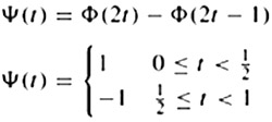
where ψa,b(t) is known as the basis function, which is a time dilation and translation version of a bandpass signal Ψ(t), called the mother wavelet and is defined as:
| (4.12) |
where a and b are time dilation and translation parameters, respectively. The effects of these parameters are shown in Figure 4.5.
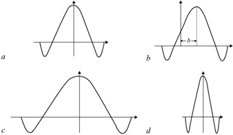
Figure 4.5: Effect of time dilation and translation on the mother wavelet (a) mother wavelet Ψ(t) = Ψ1,0(t), a = 1, b = 0 (b) wavelet Ψ1,b(t), a = 1, b ≠ 0 (c) wavelet Ψ 2,0(t) at scale a = 2, b = 0 (d) wavelet Ψ 0.5,0(t) at scale a = 1/2, b = 0
The width of the basis function varies with the dilation factor (or scale) a. The larger is a, the wider becomes the basis function in the time domain and hence narrower in the frequency domain. Thus it allows varying time and frequency resolutions (with trade-off between both) in the wavelet transform. It is this property of the wavelet transform that makes it suitable for analysing signals having features of different sizes as present in natural images. For each feature size, there is a basis function Ψa,b(t) in which it will be best analysed. For example: in a picture of a house with a person looking through a window, the basis function with larger a will analyse conveniently the house as a whole. The person by the window will be best analysed at a smaller scale and the eyes of the person at even smaller scale. So the wavelet transform is analogous to the analysis of a signal in the frequency domain using bandpass filters of variable central frequency (which depends on parameter a) but with a constant quality factor. Note that in filters, the quality factor is the ratio of the centre frequency to the bandwidth of the filter.
4.3.1 Discrete wavelet transform (DWT)
As the wavelet transform defined in eqn. 4.11 maps a one-dimensional signal x(t) into a two-dimensional function Xw(a, b), this increase in dimensionality makes it extremely redundant, and the original signal can be recovered from the wavelet transform computed on the discrete values of a and b [9]. The a can be made discrete by choosing ![]() , with a0 > 1 and m an integer. As a increases, the bandwidth of the basis function (or frequency resolution) decreases and hence more resolution cells are needed to cover the region. Similarly, making b discrete corresponds to sampling in time (sampling frequency depends on the bandwidth of the signal to be sampled which in turn is inversely proportional to a), it can be chosen as
, with a0 > 1 and m an integer. As a increases, the bandwidth of the basis function (or frequency resolution) decreases and hence more resolution cells are needed to cover the region. Similarly, making b discrete corresponds to sampling in time (sampling frequency depends on the bandwidth of the signal to be sampled which in turn is inversely proportional to a), it can be chosen as ![]() . For a0 = 2 and b0 = 1 there are choices of Ψ(t) such that the function Ψm,n(t) forms an orthonormal basis of space of square integrable functions. This implies that any square integrable function x(t) can be represented as a linear combination of basis functions as:
. For a0 = 2 and b0 = 1 there are choices of Ψ(t) such that the function Ψm,n(t) forms an orthonormal basis of space of square integrable functions. This implies that any square integrable function x(t) can be represented as a linear combination of basis functions as:
| (4.13) | 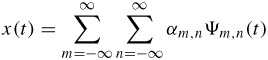 |
where αm,n are known as the wavelet transform coefficients of x(t) and are obtained from eqn. 4.11 by:
| (4.14) | 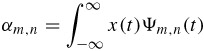 |
It is interesting to note that for every increment in m, the value of a doubles. This implies doubling the width in the time domain and halving the width in the frequency domain. This is equivalent to signal analysis with octave band decomposition and corresponds to dyadic wavelet transform similar to that shown in Figure 4.1, used to describe the basic principles of subband coding, and hence the wavelet transform is a type of subband coding.
4.3.2 Multiresolution representation
Application of the wavelet transform to image coding can be better understood with the notion of multiresolution signal analysis. Suppose there is a function Φ(t) such that the set Φ (t - n), n ∈ Z is orthonormal. Also suppose Φ(t) is the solution of a two-scale difference equation:
| (4.15) | 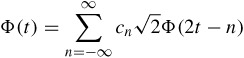 |
where
| (4.16) |
Let x(t) be a square integrable function, which can be represented as a linear combination of Φ(t - n) as:
| (4.17) | 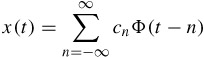 |
where cn is the expansion coefficient and is the projection of x(t) onto Φ(t - n). Since dilation of a function varies its resolution, it is possible to represent x(t) at various resolutions by dilating and contracting the function Φ(t). Thus x(t) at any resolution m can be represented as:
| (4.18) |
If Vm is the space generated by 2-m/2Φ(2-mt - n), then from eqn. 4.15, Φ(t) is such that for any i > j, the function that generates space Vi is also in Vj, i.e. Vi ⊂ Vj (i > j). Thus spaces at successive scales can be nested such that Vm for increasing m can be viewed as the space of decreasing resolution. Therefore, a space at a coarser resolution Vj-1 can be decomposed into two subspaces: a space at a finer resolution Vj and an orthogonal complement of Vj, represented by Wj such that Vj + Wj = Vj-1 where Wj ⊥ Vj. The space Wj is the space of differences between the coarser and the finer scale resolutions, which can be seen as the amount of detail added when going from a smaller resolution Vj to a larger resolution Vj-1. The hierarchy of spaces is depicted in Figure 4.6.
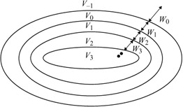
Figure 4.6: Multiresolution spaces
Mallat [10] has shown that in general the basis for Wj consists in translations and dilations of a single prototype function Ψ (t), called a wavelet. Thus, Wm is the space generated by Ψm,n(t) = 2-m/2Ψ(2-m t - n). The wavelet Ψ(t) ∈ V_1 can be obtained from Φ(t) as:
| (4.19) |  |
The function Φ(t) is called the scaling function of the multiresolution representation. Thus the wavelet transform coefficients of eqn. 4.14 correspond to the projection of x(t) onto a detail space of resolution m, Wm. Hence, a wavelet transform basically decomposes a signal into spaces of different resolutions. In the literature, these kinds of decomposition are in general referred to as multiresolution decomposition. Here is an example of calculating the Haar wavelet through this technique.
Example: Haar wavelet
The scaling function of the Haar wavelet is the well known rectangular (rect) function:
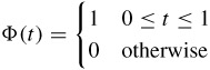
The rect function satisfies eqn. 4.15 with cn calculated from eqn. 4.16 as:
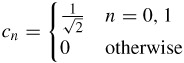
Thus using eqn. 4.19, the Haar wavelet can be found as:
The scaling function Φ(t) (a rect function) and the corresponding Haar wavelet Ψ(t) for this example are shown in Figure 4.7a and b, respectively. In terms of the approximation perspective, the multiresolution decomposition can be explained as follows. Let x(t) be approximated at resolution j by function Ajx(t) through the expansion series of the orthogonal basis functions. Since Wj represents the space of difference between a coarser scale Vj_1 and a finer scale Vj, then Djx(t) ∈ Wj represents the difference of approximation of x(t) at the j - 1th and jth resolution (i.e. Djx(t) = Aj-1x(t) - Ajx(t)).
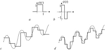
Figure 4.7: (a) Haar scaling function (b) Haar wavelet (c) approximation of a continuous function, x(t), at coarser resolution A0x(t) (d) higher resolution approximation A1x(t)
Thus the signal x(t) can be split as x(t) = A-1x(t) = A0x(t) + D0x(t).
Figure 4.7c and d show the approximations of a continuous function at the two successive resolutions using a rectangular scaling function. The coarser approximation A0x(t) is shown in Figure 4.7c and at higher resolution approximation A1x(t) in Figure 4.7d where the scaling function is a dilated version of the rectangular function. For a smooth function x(t), most of the variation (signal energy) is contained in A0x(t), and D0x(t) is nearly zero. By repeating this splitting procedure and partitioning A0x(t) = A1x(t) + D1x(t), the wavelet transform of signal x(t) can
be obtained and hence the original function x(t) can be represented in terms of its wavelets as:
| (4.20) |
where n represents the number of decompositions. Since the dynamic ranges of the detail signals Djx(t) are much smaller than the original function x(t), they are easier to code than the coefficients in the series expansion of eqn. 4.13.
4.3.3 Wavelet transform and filter banks
For the repeated splitting procedure described above to be practical, there should be an efficient algorithm for obtaining Djx(t) from the original expansion coefficient of x(t). One of the consequences of multiresolution space partitioning is that the scaling function Φ(t) possesses a self similarity property. If Φ(t) and ![]() are the analysis and synthesis scaling functions, and Ψ(t) and
are the analysis and synthesis scaling functions, and Ψ(t) and ![]() are analysis and synthesis wavelets, then since Vj ⊂ Vj-1, these functions can be recursively defined as:
are analysis and synthesis wavelets, then since Vj ⊂ Vj-1, these functions can be recursively defined as:
| (4.21) | 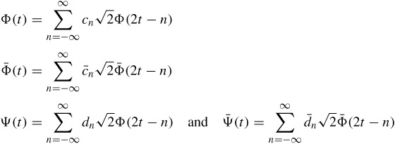 |
These recurrence relations provide ways of calculating the coefficients of the approximation of x(t) at resolution j, Ajx(t), and the coefficients of the detail signal Djx(t) from the coefficients of the approximation of x(t) at a higher resolution Aj-1x(t). In fact, simple mathematical manipulations can reveal that both the coefficients of approximation at a finer resolution and detail coefficients can be obtained by convolving the coefficient of approximation at a coarser resolution with a filter and downsampling it by a factor of 2. For a lower resolution approximation coefficient, the filter is a lowpass filter with taps hk = c_k, and for the details the filter is a highpass filter with taps gk = d_k. Inversely, the signal at a higher resolution can be recovered from its approximation at a lower resolution and coefficients of the corresponding detail signal. It can be accomplished by upsampling the coefficients of approximation at a lower resolution and detail coefficients by a factor of 2, convolving them with the synthesis filters of taps ![]() and
and ![]() , respectively, and adding them together. One step of splitting and inverse process is shown in Figure 4.8, which is in fact the same as Figure 4.3 for subband. Thus the filtering process splits the signals into lowpass and highpass frequency components and hence increases frequency resolution by a factor of 2, but downsampling reduces the temporal resolution by the same factor. Hence, at each successive step, better frequency resolution at the expense of temporal resolution is achieved.
, respectively, and adding them together. One step of splitting and inverse process is shown in Figure 4.8, which is in fact the same as Figure 4.3 for subband. Thus the filtering process splits the signals into lowpass and highpass frequency components and hence increases frequency resolution by a factor of 2, but downsampling reduces the temporal resolution by the same factor. Hence, at each successive step, better frequency resolution at the expense of temporal resolution is achieved.
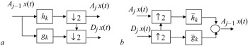
Figure 4.8: One stage wavelet transform (a) analysis (b) synthesis
4.3.4 Higher order systems
The multidimensional wavelet transform can be obtained by extending the concept of the two-band filter structure of Figure 4.8 in each dimension. For example, decomposition of a two-dimensional image can be performed by carrying out one-dimensional decomposition in the horizontal and then in the vertical directions.
A seven-band wavelet transform coding of this type is illustrated in Figure 4.9, where band splitting is carried out alternately in the horizontal and vertical directions. In the Figure, L and H represent the lowpass and highpass analysis filters with a 2:1 downsampling, respectively. At the first stage of dyadic decomposition, three subimages with high frequency contents are generated. The subimage LH1 has mainly low horizontal, but high vertical frequency image details. This is reversed in the HL1 subimage. The HH1 subimage has high horizontal and high vertical image details. These image details at a lower frequency are represented by the LH2, HL2 and HH2 bands, respectively. The LL2 band is a lowpass subsampled image, which is a replica of the original image, but at a smaller size.
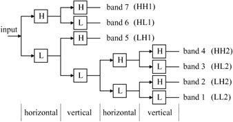
Figure 4.9: Multiband wavelet transform coding using repeated two-band splits
4.3.5 Wavelet filter design
As we saw in section 4.3.3, in practice the wavelet transform can be realised by a set of filter banks, similar to those of the subband. Relations between the analysis and synthesis of the scaling and wavelet functions also follow those of the synthesis and analysis filters of the subband. Hence we can use the concept of the product filter, defined in eqn. 4.7, to design wavelet filters. However, if we use the product filter as was used for the subband, we do not achieve anything new. But, if we add some constraints on the product filter, such that the property of the wavelet transform is maintained, then a set of wavelet filters can be designed.
One of the constraints required to be imposed on the product filter P(z) is that the resultant filters H0(z) and H1(z) be continuous, as required by the wavelet definition. Moreover, it is sometimes desirable to have wavelets with the largest possible number of continuous derivatives. This property in terms of the z transform means that the wavelet filters and consequently the product filter should have zeros at z = -1. A measure of the number of derivatives or number of zeros at z = -1 is given by the regularity of the wavelets and also called the number of vanishing moments [11]. This means that in order to have regular filters, filters must have a sufficient number of zeros at z = -1, the larger the number of zeros, the more regular the filter is.
Also since, in images, phase carries important information it is necessary that filters must have linear phase responses. On the other hand, although the orthogonal filters have an energy preserving property, most of the orthogonal filters do not have phase linearity. A particular class of filters that have linear phase in both their analysis and synthesis and are very close to orthogonal are known as biorthogonal filters. In biorthogonal filters, the lowpass analysis and the highpass synthesis filters are orthogonal to each other and similarly the highpass analysis and the lowpass synthesis are orthogonal to each other, hence the name biorthogonal. Note that, in the biorthogonal filters, since the lowpass and the highpass of either analysis or synthesis filters can be of different lengths, they are not themselves orthogonal to each other.
Thus for a wavelet filter to have at least n zeros at z = -1, we chose the product filter to be [12]:
| (4.22) |
where Q(z) has n unknown coefficients. Depending on the choice of Q(z) and the regularity of the desired wavelets, one can design a set of wavelets as desired. For example with:
n = 2 and Q(z) = -1 + 4z-1 - z-2
the product filter becomes:
| (4.23) |
and with a proper weighting for orthonormality and then factorisation, it leads to two sets of (5, 3) and (4, 4) filter banks of eqn. 4.10. The weighting factor is determined from eqn. 4.7. These filters were originally derived for subbands, but as we see they can also be used for wavelets. Filter pair (5, 3) is the recommended filter for the lossless image coding in JPEG2000 [13]. The coefficients of its analysis filters are given in Table 4.1.
| n | lowpass | highpass |
|---|---|---|
| 0 | 6/8 | +1 |
| ±1 | 2/8 | -1/2 |
| ±2 | -1/8 |
As another example with:
| (4.24) | 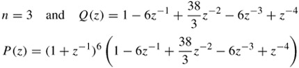 |
the (9,3) pair of Daubechies filters [9] can be derived, which are given in Table 4.2. These filter banks are recommended for still image coding in MPEG-4 [14].
| n | lowpass | highpass |
|---|---|---|
| 0 | 0.99436891104360 | 0.70710678118655 |
| ±1 | 0.41984465132952 | -0.35355339059327 |
| ±2 | -0.17677669529665 | |
| ±3 | -0.06629126073624 | |
| ±4 | 0.03314563036812 |
Another popular biorthogonal filter is the Duabechies (9,7) filter bank, recommended for lossy image coding in the JPEG2000 standard [13]. The coefficients of its lowpass and highpass analysis filters are tabulated in Table 4.3. These filters are known to have the highest compression efficiency.
| n | lowpass | highpass |
|---|---|---|
| 0 | 0.85269865321930 | -0.7884848720618 |
| ±1 | 0.37740268810913 | 0.41809244072573 |
| ±2 | -0.11062402748951 | 0.04068975261660 |
| ±3 | -0.02384929751586 | -0.06453905013246 |
| ±4 | 0.03782879857992 |
The corresponding lowpass and highpass synthesis filters can be derived from the above analysis filters, using the relationship between the synthesis and analysis filters given by eqn. 4.4. That is G0(z) = H1(-z) and G1(z) = -H0(-z).
Example
As an example of the wavelet transform, Figure 4.10 shows all the seven subimages generated by the encoder of Figure 4.9 for a single frame of the flower garden test sequence, with a nine-tap low and three-tap highpass analysis Daubechies filter pair, (9, 3), given in Table 4.2. These filters have been recommended for coding of still images in MPEG-4 [14], which has been shown to achieve good compression efficiency.
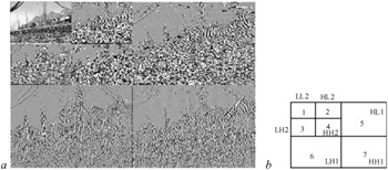
Figure 4.10: (a) the seven subimages generated by the encoder of Figure 4.9 (b) layout of individual bands
The original image (not shown) dimensions were 352 pixels by 240 lines. Bands 1–4, at two levels of subdivision, are 88 by 60, and bands 5–7 are 176 by 120 pixels. All bands but band 1 (LL2) have been amplified by a factor of four and an offset of +128 to enhance visibility of the low level details they contain. The scope for bandwidth compression arises mainly from the low energy levels that appear in the highpass subimages.
Since at image borders all the input pixels are not available, a symmetric extension of the input texture is performed before applying the wavelet transform at each level [14]. The type of symmetric extension can vary. For example in MPEG-4, to satisfy the perfect reconstruction conditions with the Daubechies (9, 3) tap analysis filter pairs, two types of symmetric extension are used.
Type A is only used at the synthesis stage. It is used at the trailing edge of lowpass filtering and the leading edge of highpass filtering stages. If the pixels at the boundary of the objects are represented by abcde, then the type A extension becomes edcba|abcde, where the letters in bold type are the original pixels and those in plain are the extended pixels. Note that for a (9,3) analysis filter pair of Table 4.2, the synthesis filter pair will be (3, 9) with G0(z) = H1(-z) and G1(z) = -H0(-z), as was shown in eqn. 4.4.
Type B extension is used for both leading and trailing edges of the low and highpass analysis filters. For the synthesis filters, it is used at the leading edge of the lowpass, but at the trailing edge of the highpass. With this type of extension, the extended pixels at the leading and trailing edges become edcb|abcde and abcde|dcba, respectively.
EAN: 2147483647
Pages: 148