4.2 Subband coding

4.2 Subband coding

Before describing the wavelet transform, let us look at its predecessor, subband coding, which sometimes is called the early wavelet transform [5]. As we will see later, in terms of image coding they are similar. However, subband coding is a product designed by engineers [6], and the wavelet transform was introduced by mathematicians [7]. Therefore before proceeding to mathematics, which is sometimes cumbersome to follow, an engineering view of multiresolution signal processing may help us to understand it better.

Subband coding was first introduced by Crochiere et al. in 1976 [6], and has since proved to be a simple and powerful technique for speech and image compression. The basic principle is the partitioning of the signal spectrum into several frequency bands, then coding and transmitting each band separately. This is particularly suited to image coding. First, natural images tend to have a nonuniform frequency spectrum, with most of the energy being concentrated in the lower frequency band. Secondly, human perception of noise tends to fall off at both high and low frequencies and this enables the designer to adjust the compression distortion according to perceptual criteria. Thirdly, since images are processed in their entirety, and not in artificial blocks, there is no block structure distortion in the coded picture, as occurs in the block-transform-based image encoders, such as DCT.

Thus subband, like the Fourier transform, is based on frequency domain analysis of the image but its filter banks have a better decorrelation property that suits natural images better. This can be explained as follows. Fourier basis functions are very exact in frequency, but are spatially not precise. In other words, the signal energy of Fourier basis functions is not concentrated at one frequency, but is spread over all space. This would not be a problem if image pixels were always correlated. However, in reality, pixels in images of interest generally have low correlation, especially across the image discontinuities such as edges. In contrast to Fourier basis functions, the subband bases not only have fairly good frequency concentration but are also spatially compact. If image edges are not too closely packed, most of the subband basis elements will not intersect with them, thus performing a better decorrelation on average.

In subband coding the band splitting is done by passing the image data through a bank of bandpass analysis filters, as shown in Figure 4.1. In order to adapt the frequency response of the decomposed pictures to the characteristics of the human visual system, filters are arranged into octave bands.

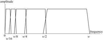
Figure 4.1: A bank of bandpass filters

Since the bandwidth of each filtered version of the image is reduced, they can now in theory be downsampled at a lower rate, according to the Nyquist criteria, giving a series of reduced size subimages. The subimages are then quantised, coded and transmitted. The received subimages are restored to their original sizes and passed through a bank of synthesis filters, where they are interpolated and added to reconstruct the image.

In the absence of quantisation error, it is required that the reconstructed picture should be an exact replica of the input picture. This can only be achieved if the spatial frequency response of the analysis filters tiles the spectrum (i.e. the individual bands are set one after the other) without overlapping, which requires infinitely sharp transition regions and cannot be realised practically. Instead, the analysis filter responses have finite transition regions and do overlap, as shown in Figure 4.1, which means that the downsampling/upsampling processes introduce aliasing distortion into the reconstructed picture.

In order to eliminate the aliasing distortion, the synthesis and analysis filters have to have certain relationships such that the aliased components in the transition regions cancel each other out. To see how such a relation can make alias-free subband coding possible, consider a two-band subband, as shown in Figure 4.2.

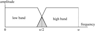
Figure 4.2: A two-band analysis filter

The corresponding two-band subband encoder/decoder is shown in Figure 4.3. In this diagram, filters H₀(z) and H₁(z) represent the z transform transfer functions of the respective lowpass and highpass analysis filters. Filters G₀(z) and G₁(z) are the corresponding synthesis filters. The downsampling and upsampling factors are 2.

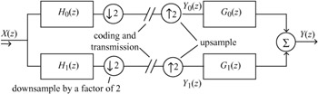
Figure 4.3: A two-band subband encoder/decoder

At the encoder, downsampling by 2 is carried out by discarding alternate samples, the remainder being compressed into half the distance occupied by the original sequence. This is equivalent to compressing the source image by a factor of 2, which doubles all the frequency components present. The frequency domain effect of this downsampling/compression is thus to double the width of all components in the sampled spectrum.

At the decoder, the upsampling is a complementary procedure: it is achieved by inserting a zero-valued sample between each input sample, and is equivalent to a spatial expansion of the input sequence. In the frequency domain, the effect is as usual the reverse and all components are compressed towards zero frequency.

The problem with these operations is the impossibility of constructing ideal, sharp cut analysis filters. This is illustrated in Figure 4.4a. Spectrum A shows the original sampled signal which has been lowpass filtered so that some energy remains above F_s/4, the cutoff of the ideal filter for the task. Downsampling compresses the signal and expands to give B, and C is the picture after expansion or upsampling. As well as those at multiples of F_s, this process generates additional spectrum components at odd multiples of F_s/2. These cause aliasing when the final subband recovery takes place as at D.

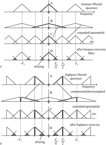
Figure 4.4: (a) lowpass subband generation and recovery (b) highpass subband generation and recovery

In the highpass case, Figure 4.4b, the same phenomena occur, so that on recovery there is aliased energy in the region of F_s/4. The final output image is generated by adding the lowpass and highpass subbands regenerated by the upsamplers and associated filters. The aliased energy would normally be expected to cause interference. However, if the phases of the aliased components from the high and lowpass sub-bands can be made to differ by π, then cancellation occurs and the recovered signal is alias free.

How this can be arranged is best analysed by reference to z transforms. Referring to Figure 4.3, after the synthesis filters, the reconstructed output in z transform notation can be written as:

(4.1) 

where Y₀(z) and Y₁(z) are inputs to the synthesis filters after upsampling. Assuming there are no quantisation and transmission errors, the reconstructed samples are given by:

(4.2)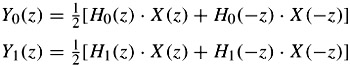 

where the aliasing components from the downsampling of the lower and higher bands are given by H₀(-z)X(-z) and H₁(-z)X (-z), respectively. By substituting these two equations in the previous one, we get:

(4.3)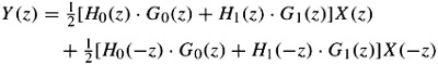 

The first term is the desired reconstructed signal, and the second term is aliased components. The aliased components can be eliminated regardless of the amount of overlap in the analysis filters by defining the synthesis filters as:

(4.4) 

With such a relation between the synthesis and analysis filters, the reconstructed signal now becomes:

(4.5) 

If we define P(z) = H₀(z)H₁(-z), then the reconstructed signal can be written as:

(4.6) 

Now the reconstructed signal can be a perfect, but an m-sample delayed, replica of the input signal if:

(4.7) 

Thus the z transform input/output signals are given by:

(4.8) 

This relation in the pixel domain implies that the reconstructed pixel sequence {y(n)} is an exact replica of the input sequence but delayed by m pixels, {i.e. x(n - m)}.

In these equations P(z) is called the product filter and m is the delay introduced by the filter banks. The design of analysis/synthesis filters is based on factorisation of the product filter P(z) into linear phase components H₀(z) and H₁(-z), with the constraint that the difference between the product filter and its image should be a simple delay. Then the product filter must have an odd number of coefficients. LeGall and Tabatabai [8] have used a product filter P(z) of the kind:

(4.9) 

and by factorising have obtained several solutions for each pair of the analysis and synthesis filters:

(4.10)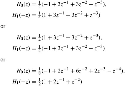 

The synthesis filters G₀(z) and G₁(z) are then derived using their relations with the analysis filters, according to eqn. 4.4. Each of the above equation pairs gives the results P(z) - P(-z) = 2z^-3, which implies that the reconstruction is perfect with a delay of three samples.