3.4 Variable length coding
3.4 Variable length coding
For further bit rate reduction, the transform coefficients and the coordinates of the motion vectors are variable length coded (VLC). In VLC, short code words are assigned to the highly probable values and long code words to the less probable ones. The lengths of the codes should vary inversely with the probability of occurrences of the various symbols in VLC. The bit rate required to code these symbols is the inverse of the logarithm of probability, p, at base 2 (bits), i.e. log2 p. Hence, the entropy of the symbols which is the minimum average bits required to code the symbols can be calculated as:
| (3.9) |  |
There are two types of VLC, which are employed in the standard video codecs. They are Huffman coding and arithmetic coding. It is noted that Huffman coding is a simple VLC code, but its compression can never reach as low as the entropy due to the constraint that the assigned symbols must have an integral number of bits. However, arithmetic coding can approach the entropy since the symbols are not coded individually [14]. Huffman coding is employed in all standard codecs to encode the quantised DCT coefficients as well as motion vectors. Arithmetic coding is used, for example, in JPEG, JPEG2000, H.263 and shape and still image coding of MPEG-4 [15–17], where extra compression is demanded.
3.4.1 Huffman coding
Huffman coding is the most commonly known variable length coding method based on probability statistics. Huffman coding assigns an output code to each symbol with the output codes being as short as 1 bit, or considerably longer than the input symbols, depending on their probability. The optimal number of bits to be used for each symbol is - log2 p, where p is the probability of a given symbol.
However, since the assigned code words have to consist of an integral number of bits, this makes Huffman coding suboptimum. For example, if the probability of a symbol is 0.33, the optimum number of bits to code that symbol is around 1.6 bits, but the Huffman coding scheme has to assign either one or two bits to the code. In either case, on average it will lead to more bits compared to its entropy. As the probability of a symbol becomes very high, Huffman coding becomes very nonoptimal. For example, for a symbol with a probability of 0.9, the optimal code size should be 0.15 bits, but Huffman coding assigns a minimum value of one bit code to the symbol, which is six times larger than necessary. Hence, it can be seen that resources are wasted.
To generate the Huffman code for symbols with a known probability of occurrence, the following steps are carried out:
-
rank all the symbols in the order of their probability of occurrence
-
successively merge every two symbols with the least probability to form a new composite symbol, and rerank order them; this will generate a tree, where each node is the probability of all nodes beneath it
-
trace a path to each leaf, noting the direction at each node.
Figure 3.10 shows an example of Huffman coding of seven symbols, A-G. Their probabilities in descending order are shown in the third column. In the next column the two smallest probabilities are added and the combined probability is included in the new order. The procedure continues to the last column, where a single probability of 1 is reached. Starting from the last column, for every branch of probability a 0 is assigned on the top and a 1 in the bottom, shown in bold digits in the Figure. The corresponding codeword (shown in the first column) is read off by following the sequence from right to left. Although with fixed word length each sample is represented by three bits, they are represented in VLC from two to four bits.
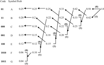
Figure 3.10: An example of Huffman code for seven symbols
The average bit per symbol is then:
0.25 × 2 + 0.20×2 + 0.18×3 + 0.15×3 + 0.12×3 + 0.06×4 + 0.04×4 = 2.65 bits
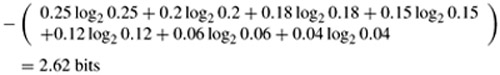
which is very close to the entropy given by:
It should be noted that for a large number of symbols, such as the values of DCT coefficients, such a method can lead to a long string of bits for the very rarely occurring values, and is impractical. In such cases normally a group of symbols is represented by their aggregate probabilities and the combined probabilities are Huffman coded, the so-called modified Huffman code. This method is used in JPEG. Another method, which is used in H.261 and MPEG, is two-dimensional Huffman, or three-dimensional Huffman in H.263 [9,16].
3.4.2 Arithmetic coding
Huffman coding can be optimum if the symbol probability is an integer power of ![]() , which is usually not the case. Arithmetic coding is a data compression technique that encodes data by creating a code string, which represents a fractional value on the number line between 0 and 1 [14]. It encourages clear separation between the model for representing data and the encoding of information with respect to that model. Another advantage of arithmetic coding is that it dispenses with the restriction that each symbol must translate into an integral number of bits, thereby coding more efficiently. It actually achieves the theoretical entropy bound to compression efficiency for any source. In other words, arithmetic coding is a practical way of implementing entropy coding.
, which is usually not the case. Arithmetic coding is a data compression technique that encodes data by creating a code string, which represents a fractional value on the number line between 0 and 1 [14]. It encourages clear separation between the model for representing data and the encoding of information with respect to that model. Another advantage of arithmetic coding is that it dispenses with the restriction that each symbol must translate into an integral number of bits, thereby coding more efficiently. It actually achieves the theoretical entropy bound to compression efficiency for any source. In other words, arithmetic coding is a practical way of implementing entropy coding.
There are two types of modelling used in arithmetic coding: the fixed model and the adaptive model. Modelling is a way of calculating, in any given context, the distribution of probabilities for the next symbol to be coded. It must be possible for the decoder to produce exactly the same probability distribution in the same context. Note that probabilities in the model are represented as integer frequency counts. Unlike the Huffman-type, arithmetic coding accommodates adaptive models easily and is computationally efficient. The reason why data compression requires adaptive coding is that the input data source may change during encoding, due to motion and texture.
In the fixed model, both encoder and decoder know the assigned probability to each symbol. These probabilities can be determined by measuring frequencies in representative samples to be coded and the symbol frequencies remain fixed. Fixed models are effective when the characteristics of the data source are close to the model and have little fluctuation.
In the adaptive model, the assigned probabilities may change as each symbol is coded, based on the symbol frequencies seen so far. Each symbol is treated as an individual unit and hence there is no need for a representative sample of text. Initially, all the counts might be the same, but they update, as each symbol is seen, to approximate the observed frequencies. The model updates the inherent distribution so the prediction of the next symbol should be close to the real distribution mean, making the path from the symbol to the root shorter.
Due to the important role of arithmetic coding in the advanced video coding techniques, in the following sections a more detailed description of this coding technique is given.
3.4.2.1 Principles of arithmetic coding
The fundamental idea of arithmetic coding is to use a scale in which the coding intervals of real numbers between 0 and 1 are represented. This is in fact the cumulative probability density function of all the symbols which add up to 1. The interval needed to represent the message becomes smaller as the message becomes longer, and the number of bits needed to specify that interval is increased. According to the symbol probabilities generated by the model, the size of the interval is reduced by successive symbols of the message. The more likely symbols reduce the range less than the less likely ones and hence they contribute fewer bits to the message.
To explain how arithmetic coding works, a fixed model arithmetic code is used in the example for easy illustration. Suppose the alphabet is {a, e, i, o, u, !} and the fixed model is used with the probabilities shown in Table 3.4.
| Symbol | Probability | Range |
|---|---|---|
| a | 0.2 | [0.0, 0.2) |
| e | 0.3 | [0.2, 0.5) |
| i | 0.1 | [0.5, 0.6) |
| o | 0.2 | [0.6, 0.8) |
| u | 0.1 | [0.8, 0.9) |
| ! | 0.1 | [0.9, 1.0) |
Once the symbol probability is known, each individual symbol needs to be assigned a portion of the [0, 1) range that corresponds to its probability of appearance in the cumulative density function. Note also that the character with a range of [lower, upper) owns everything from lower up to, but not including, the upper value. So, the alphabet u with probability 0.1, defined in the cumulative range of [0.8, 0.9), can take any value from 0.8 to 0.8999 ....
The most significant portion of an arithmetic coded message is the first symbol to be encoded. Using an example that a message eaii! is to be coded, the first symbol to be coded is e. Hence, the final coded message has to be a number greater than or equal to 0.2 and less than 0.5. After the first character is encoded, we know that the lower number and the upper number now bound our range for the output. Each new symbol to be encoded will further restrict the possible range of the output number during the rest of the encoding process.
The next character to be encoded, a, is in the range of 0-0.2 in the new interval. It is not the first number to be encoded, so it belongs to the range corresponding to 0-0.2, but in the new subrange of [0.2, 0.5). This means that the number is now restricted to the range of [0.2, 0.26), since the previous range was 0.3 (0.5 - 0.2 = 0.3) units long and one-fifth of that is 0.06. The next symbol to be encoded, i, is in the range of [0.5, 0.6), that corresponds to 0.5-0.6 in the new subrange of [0.2, 0.26) and gives the smaller range [0.23, 0.236). Applying this rule for coding of successive characters, Table 3.5 shows the successive build up of the range of the message coded so far.
| New character | Range | |
|---|---|---|
| Initially: | [0, 1) | |
| After seeing a symbol: | e | [0.2, 0.5) |
| a | [0.2, 0.26) | |
| i | [0.23, 0.236) | |
| i | [0.233, 0.2336) | |
| ! | [0.23354, 0.2336) |
Figure 3.11 shows another representation of the encoding process. The range is expanded to fill the whole range at every stage and marked with a scale that gives the end points as a number. The final range, [0.23354, 0.2336) represents the message eaii!. This means that if we transmit any number in the range of 0.23354 ≤ x < 0.2336, that number represents the whole message of eaii!.
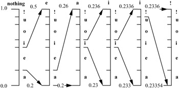
Figure 3.11: Representation of arithmetic coding process with the interval scaled up at each stage for the message eaii!
Given this encoding scheme, it is relatively easy to see how during the decoding the individual elements of the eaii! message are decoded. To verify this, suppose a number x = 0.23355 in the range of 0.23354 ≤ x < 0.2336 is transmitted. The decoder, using the same probability intervals as the encoder, performs a similar procedure. Starting with the initial interval [0, 1), only the interval [0.2, 0.5) of e envelops the transmitted code of 0.23355. So the first symbol can only be e. Similar to the encoding process, the symbol intervals are then defined in the new interval [0.2, 0.5). This is equivalent to defining the code within the initial range [0, 1), but offsetting the code by the lower value and then scaling up within its original range. That is, the new code will be (0.23355 - 0.2)/(0.5 - 0.2) = 0.11185, which is enveloped by the interval [0.0, 0.2) of symbol a. Thus the second decoded symbol is a. To find the third symbol, a new code within the range of a should be found, i.e. (0.11185 - 0.0)/(0.2 - 0.0) = 0.55925. This code is enveloped by the range of [0.5, 0.6) of symbol i and the resulting new code after decoding the third symbol will be (0.55925 - 0.5)/(0.6 - 0.5) = 0.5925, which is again enveloped by [0.5, 0.6). Hence the fourth symbol will be i. Repeating this procedure will yield a new code of (0.5925 - 0.5)/(0.6 - 0.5) = 0.925. This code is enveloped by [0.9, 1), which decodes symbol !, the end of decoding symbol, and the decoding process is terminated. Table 3.6 shows the whole decoding process of the message eaii!.
| Encoded number | Output symbol | Range |
|---|---|---|
| 0.23355 | e | [0.2, 0.5) |
| 0.11185 | a | [0.0, 0.2) |
| 0.55925 | i | [0.5, 0.6) |
| 0.59250 | i | [0.5, 0.6) |
| 0.92500 | ! | [0.9, 1.0) |
In general, the decoding process can be formulated as:
| (3.10) |
where Rn is a code within the range of lower value Ln and upper value Un of the nth symbol and Rn+1 is the code for the next symbol.
3.4.2.2 Binary arithmetic coding
In the preceding section we saw that, as the number of symbols in the message increases, the range of the message becomes smaller. If we continue coding more symbols then the final range may even become smaller than the precision of any computer to define such a range. To resolve this problem we can work with binary arithmetic coding.
In Figure 3.11 we saw that after each stage of coding, if we expand the range to its full range of [0, 1), the apparent range is increased. However, the values of the lower and upper numbers are still small. Therefore, if the initial range of [0, 1) is replaced by a larger range of [0, MAX_VAL), where MAX_VAL is the largest integer number that a computer can handle, then the precision problem is resolved. If we use 16-bit integer numbers, then MAX_VAL= 216 - 1. Hence, rather than defining the cumulative probability in the range of [0,1), we define their cumulative frequencies scaled up within the range of [0, 216 - 1).
At the start, the coding interval [lower, upper) is initialised to the whole scale [0, MAX_VAL). The model's frequencies, representing the probability of each symbol in this range, are also set to their initial values in the range. To encode a new symbol element ek assuming that symbols e1... ek-1 have already being coded, we project the model scale to the interval resulting from the sequence of events. The new interval [lower', upper') for the sequence e1... ek is calculated from the old interval [lower, upper) of the sequence e1 ... ek-1 as follows:
| lower' | = lower + width * low/maxfreq |
| width' | = width * symb_width/maxfreq |
| upper' | = lower' + width' |
| = lower + width * (low + symb_width)/maxfreq | |
| = lower + width * up/maxfreq |
with:
-
width = upper - lower (old interval)
-
width' = upper' - lower' (new interval)
-
symb_width = up - low (model's frequency)
At this stage of the coding process, we do not need to keep the previous interval [lower, upper) in the memory, so we allocate the new values [lower', upper'). We then compare the new interval with the scale [0, MAX_VAL) to determine whether there is any bit for transmission down the channel. These bits are due to the redundancy in the binary representation of lower and upper values. For example, if values of both lower and upper are less than half the [0, MAX_VAL) range, then their most significant number in binary form is 0. Similarly, if both belong to the upper half range, their most significant number is 1. Hence we can make a general rule:
-
if lower and upper levels belong to the first half of the scale, the most significant bit for both will be 0
-
if lower and upper belong to the second half of the scale, their most significant bit will be 1
-
otherwise, when lower and upper belong to the different halves of the scale their most significant bits will be different (0 and 1).
Thus for the cases where lower and upper values have the same most significant bit, we send this bit down the channel and calculate the new interval as follows:
-
sending a 0 corresponds to removal of the second half of the scale and keeping its first half only; the new scale is expanded by a factor 2 to obtain its representation in the whole scale of [0, MAX_VAL) again, as shown in Figure 3.12
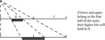
Figure 3.12: Both lower and upper values in the first half -
sending a 1 corresponds to the shift of the second half of the scale to its first half; that is subtracting half of the scale value and multiplying the result by a factor 2 to obtain its representation in the whole scale again, as shown in Figure 3.13.
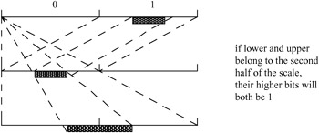
Figure 3.13: Both lower and upper values in the second half
If the interval always remains in either half of the scale after a bit has been sent, the operation is repeated as many times as necessary to obtain an interval occupying both halves of the scale. The complete procedure is called the interval testing loop.
Now we go back to the case where both of the lower and upper values are not in either of the half intervals. Here we identify two cases: first the lower value is in the second quarter of the scale and the upper value is in the third quarter. Hence the range of frequency is less than 0.5. In this case, in the binary representation, the two most significant bits are different, 01 for the lower and 10 for the upper, but we can deduce some information from them. That is, in both cases, the second bit is the complementary bit to the first. Hence, if we can find out the second bit, the previous bit is its complement. Therefore, if the second bit is 1, then the previous value should be 0, and we are in the second quarter, meaning the lower value. Similar conclusions can be drawn for the upper value.
Thus we need to divide the interval within the scale of [0, MAX_VAL) into four segments instead of two. Then the scaling and shifting for this case will be done only on the portion of the scale containing second and third quarters, as shown in Figure 3.14.
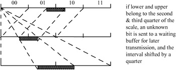
Figure 3.14: Lower and upper levels in the second and third quarter, respectively
Thus the general rule for this case is that:
-
if the interval belongs to the second and third quarters of the scale: an unknown bit ? is sent to a waiting buffer for later definition and the interval transformed as shown in Figure 3.14
-
if the interval belongs to more than two different quarters of the scale (the interval occupies parts of three or four different quarters), there is no need to transform the coding interval; the process exits from this loop and goes to the next step in the execution of the program; this means that if the probability in that interval is greater than 0.5, no bits are transmitted; this is the most important part of arithmetic coding which leads to a low bit rate.
A flow chart of the interval testing loop is shown in Figure 3.15 and a detailed example of coding a message is given in Figure 3.16. For every symbol to be coded we invoke the flow chart of Figure 3.15, except where the symbol is the end of file symbol, where the program stops. After each testing loop, the model can be updated (frequencies modified if the adaptive option has been chosen).
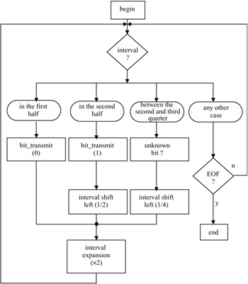
Figure 3.15: A flow chart for binary arithmetic coding
#define q1 16384 #define q2 32768 #define q3 49152 #define top 65535 static long low, high, opposite_bits, length; void encode_a_symbol (int index, int cumul_freq[]) { length = high - low +1; high = low -1 + (length * cumul_freq[index]) / cumul_freq[0] ; low += (length * cumul_freq[index+1])/ cumul_freq[0] ; for( ; ; ){ if(high <q2){ send out a bit "0" to PSC_FIFO; while (opposite_bits > 0) { send out a bit "1" to PSC_FIFO; opposite_bits--; } } else if (low >= q2) { send out a bit "1" to PSC_FIFO; while (opposite_bits > 0) { send out a bit "0" to PSC_FIFO; opposite_bits--; } low -= q2; high -= q2; } else if (low >= q1 && high < q3) { opposite_bits += 1; low -= q1; high -= q1; } else break; low *= 2; high = 2 * high + 1; } } Figure 3.16: A C program of binary arithmetic coding
A C program of binary arithmetic coding is given in Figure 3.16.
The values of low and high are initialised to 0 and top, respectively. PSC_FIFO is first-in-first-out (FIFO) for buffering the output bits from the arithmetic encoder. The model is specified through cumul_freq [ ], and the symbol is specified using its index in the model.
3.4.2.3 An example of binary arithmetic coding
Because of the complexity of the arithmetic algorithm, a simple example is given below. To simplify the operations further, we use a fixed model with four symbols a, b, c and d, where their fixed probabilities and cumulative probabilities are given in Table 3.7, and the message sequence of events to be encoded is bbacd.
| Symbol | | cdf |
|---|---|---|
| a | 0.3 | [0.0, 0.3) |
| b | 0.5 | [0.3, 0.8) |
| c | 0.1 | [0.8, 0.9) |
| d | 0.1 | [0.9, 1.0) |
Considering what we saw earlier, we start by initialising the whole range to [0, 1). In sending b, which has a range of [0.3, 0.8), since lower = 0.3 is in the second quarter and upper = 0.8 in the fourth quarter (occupying more than two quarters) nothing is sent, and no scaling is required, as shown in Table 3.8.
| Encoding | Coding interval | Width | Bit |
|---|---|---|---|
| initialisation: | [0, 1) | 1.000 | |
| after b: | [0.3, 0.8) | 0.500 | |
| after bb: | [0.45, 0.7) | 0.250 | |
| after interval test | [0.4, 0.9) | 0.500 | ? |
| after bba: | [0.40, 0.55) | 0.150 | |
| after interval test | [0.3, 0.6) | 0.300 | ? |
| after interval test | [0.1, 0.7) | 0.600 | ? |
| after bbac: | [0.58, 0.64) | 0.060 | |
| after interval test | [0.16, 0.28) | 0.120 | 1000 |
| after interval test | [0.32, 0.56) | 0.240 | 0 |
| after interval test | [0.14, 0.62) | 0.480 | ? |
| after bbacd: | [0.572, 0.620) | 0.048 | |
| after interval test | [0.144, 0.240) | 0.096 | 10 |
| after interval test | [0.288, 0.480) | 0.192 | 0 |
| after interval test | [0.576, 0.960) | 0.384 | 0 |
| after interval test | [0.152, 0.920) | 0.768 | 1 |
To send the next b, i.e. bb, since the previous width = 0.8 - 0.3 = 0.5, the new interval becomes [0.3 + 0.3 x 0.5, 0.3 + 0.8 x 0.5) = [0.45, 0.7). This time lower = 0.45 is in the second quarter but upper = 0.7 is in the third quarter, so the unknown bit ? is sent to the buffer, such that its value is to be determined later.
Note that since the range [0.45, 0.7) covers the second and third quarters, according to Figure 3.14, we have to shift both of them by a quarter (0.25) and then magnify by a factor of 2, i.e. the new interval is [(0.45 - 0.25) x 2, (0.7 - 0.25) x 2) = [0.4, 0.9) which has a width of 0.5. To code the next symbol a, the range becomes [0.4 + 0 x 0.5, 0.4 + 0.3 × 0.5) = [0.4, 0.55). Again since lower and upper are at the second and third quarters, the unknown ? is stored. According to Figure 3.14 both quarters are shifted by 0.25 and magnified by 2, [(0.4 - 0.25) × 2, (0.55 - 0.25) × 2) = [0.3, 0.6).
Again [0.3, 0.6) is in the second and third interval so another ? is stored. If we shift and magnify again [(0.3 - 0.25) × 2, (0.6 - 0.25) × 2) = [0.1, 0.7), which now lies in the first and third quarters, so nothing is sent if there is no scaling. Now if we code c, i.e. bbac, the interval becomes [0.1 + 0.8 × 0.6, 0.1 + 0.9 × 0.6) = [0.58, 0.64).
Now since [0.58, 0.64) is in the second half we send 1. We now go back and convert all ? to 000 complementary to 1. Thus we have sent 1000 so far. Note that bits belonging to ? are transmitted after finding a 1 or 0. Similarly, the subsequent symbols are coded and the final generated bit sequence becomes 1000010001. Table 3.8 shows this example in a tabular representation. A graphical representation is given in Figure 3.17.
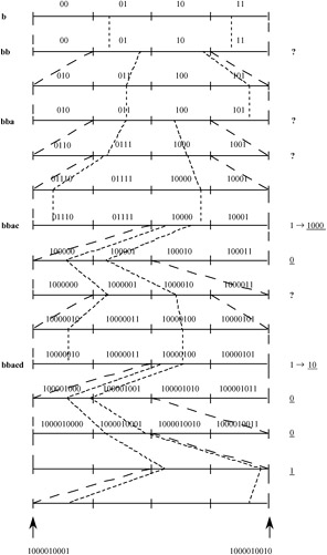
Figure 3.17: Derivation of the binary bits for the given example
3.4.2.4 Adaptive arithmetic coding
In adaptive arithmetic coding, the assigned probability to the symbols changes as each symbol is coded [18]. For binary (integer) coding, this is accomplished by assigning a frequency of 1 to each symbol at the start of the coding (initialisation). As a symbol is coded, the frequency of that symbol is incremented by one. Hence the frequencies of symbols are adapted to their number of appearances so far. The decoder follows a similar procedure. At every stage of coding, a test is done to see if the cumulative frequency (sum of the frequencies of all symbols) exceeds MAX_VAL. If this is the case, all frequencies are halved (minimum 1), and encoding continues. For a better adaptation, the frequencies of the symbols may be initialised to a predefined distribution that matches the overall statistics of the symbols better. For better results, the frequencies are updated from only the N most recently coded symbols. It has been shown that this method of adaptation with a limited past history can reduce the bit rate by more than 30 per cent below the first-order entropy of the symbols [19]. The reason for this is that, if some rare events that normally have high entropy could occur in clusters then, within only the N most recent events, they now become the more frequent events, and hence require lower bit rates.
3.4.2.5 Context-based arithmetic coding
A popular method for adaptive arithmetic coding is to adapt the assigned probability to a symbol, according to the context of its neighbours. This is called context-based arithmetic coding and forms an essential element of some image/video coding standards, such as JPEG2000 and MPEG-4. It is more efficient when it is applied to binary data, like the bit plane or the sign bits in JPEG2000 or binary shapes in MPEG-4. We explain this method with a simple example. Assume that binary symbols of a, b and c, which may take values of 0 or 1, are the three immediate neighbours of a binary symbol x, as shown in Figure 3.18.

Figure 3.18: Three immediate neighbouring symbols to x
Due to high correlation between the symbols in the image data, if the neighbouring symbols of a, b and c are mainly 1 then it is logical to assign a high probability for coding symbol x, when its value is 1. Conversely, if the neighbouring symbols are mainly 0 the assigned probability of x = 1 should be reduced. Thus we can define the context for coding a 1 symbol as:
| (3.11) |
For the binary values of a, b and c, the context has a value between 0 and 7. Higher values of the context indicate that a higher probability should be assigned for coding of 1, and a complementary probability, when the value of x is 0.
EAN: 2147483647
Pages: 148
- Chapter I e-Search: A Conceptual Framework of Online Consumer Behavior
- Chapter X Converting Browsers to Buyers: Key Considerations in Designing Business-to-Consumer Web Sites
- Chapter XIII Shopping Agent Web Sites: A Comparative Shopping Environment
- Chapter XVI Turning Web Surfers into Loyal Customers: Cognitive Lock-In Through Interface Design and Web Site Usability
- Chapter XVIII Web Systems Design, Litigation, and Online Consumer Behavior