Basic Math

Let's try something simple, shall we? If you haven't already done so, open a new spreadsheet. In cell A1, type Course Average. Select the text in the field, change the font style or size (by clicking on the font selector in the Formatting bar), and then press <Enter>. As you can see, the text is larger than the field. No problem. Place your mouse cursor on the line between the A and B cells (directly below the Formula bar). Click and hold, and then stretch the A cell to fit the text. You can do the same for the height of any given row of cells by clicking on the line between the row numbers (over to the left) and stretching these to an appropriate size.

Now move to cell A3 and type in a hypothetical number somewhere in the range of 1 100 to represent a course mark. Press <Enter> or cursor down to move to the next cell. Enter seven course marks so that cells A3 through A9 are filled. In my example, I entered 95, 67, 100, 89, 84, 79, and 93. (It seems to me that the 67 is an aberration.)

What we are going to do now is enter a formula in cell A11 to provide us with an average of all seven course scores. In cell A11, enter the following text:

 =(A3+A4+A5+A6+A7+A8+A9)/7 

When you press <Enter>, the text you entered will disappear, and instead you'll see an average for your course scores (Figure 14-2).

Figure 14-2. Setting up a simple table to determine class averages.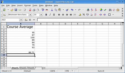

An average of 86.71 isn't a bad score (it is an A, after all). But if that 67 really was an aberration, you can easily go back to that cell, type in a different number, and press <Enter>. When you do so, the average will automagically change for you.

Calculating an average is a simple enough formula. But if I were to add 70 rows instead of 7, the resulting formula could get ugly. The beauty of spreadsheets is that they include formulas to make this whole process somewhat cleaner. For instance, I can specify a range of cells by putting a colon in between the first and last cells (A3:A9) and using a built-in function to return the average of that range. My new, improved, and cleaner formula looks like this:

 =AVERAGE (A3:A9) 

Incidentally, you can also select the cell and enter the information in the input line on the Formula bar. I mention the Formula bar for a couple of reasons. One is that you can obviously enter the information in the field as well as in the cell itself.

The second reason has to do with those little icons to the left of the input field. If you click into that input field, you'll notice that a little green checkmark will appear (to accept any changes you make to the formula), and to its left there will be a red X (to cancel the changes). Now look to the icon furthest on the left. If you hold your mouse over it, it should pop up a little tooltip that says Function Wizard. Try it. Go back to cell A11, and then click your mouse into the input field on the Formula bar. Now click on the Function Wizard icon. (You can also click Insert on the menu bar and select Function.)

On the left side you'll see a list of functions, with descriptions of those functions off to the right. For the function called AVERAGE, the description is Returns the average of a sample. Because this is what we want, click the Next button at the bottom of the window, after which you will see a window much like the one in Figure 14-3. This is where the Wizard starts to do its real work.

Figure 14-3. Using the Function Wizard to generate a function.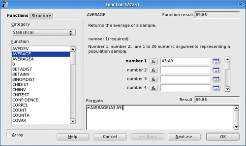

Look at the window labeled Formula at the bottom of the screen. You'll see that the formula is starting to be built. At this point, it says =AVERAGE() and nothing else. Near the middle of the screen, on the right side, are four data fields labeled number 1 through number 4. The first field is required, whereas the others are optional. You could at this point enter A3:A9, click Next, and be done. (Notice, while you are here, that the result of the formula is already displayed just above the Formula field.) Alternatively, you could click the button to the right of the number field (the tooltip will say Shrink), and the Function Wizard will shrink to a small bar floating above your spreadsheet (Figure 14-4).

Figure 14-4. The Function Wizard in a more compact format.

On your spreadsheet, select a group of fields by clicking on the first field and dragging the mouse to include all seven fields. When you let go of the mouse, the field range will have been entered for you. On the left-hand side of the shrunken Function Wizard is a maximize button (move your mouse over it to activate the tooltip). Click it, and your Wizard will return to its original size. Unless you have an additional set of fields (or you wish to create a more complex formula), click OK to complete this operation. The window will disappear, and the spreadsheet will update.