Changing Data s Appearance Based on Its Value | MicrosoftВ® Office ExcelВ® 2003 Step by Step (Step By Step (Microsoft))

Recording sales, credit limits, and other business data in a worksheet lets you make important decisions about your operations. And as you saw earlier in this chapter, you can change the appearance of data labels and the worksheet itself to make interpreting your data easier.

Another way you can make your data easier to interpret is to have Excel change the appearance of your data based on its value. These formats are called conditional formats because the data must meet certain conditions to have a format applied to it. For instance, if owner Catherine Turner wanted to highlight any Saturdays on which daily sales at The Garden Company were over $4,000, she could define a conditional format that tests the value in the cell recording total sales, and thatwill change the format of the cell s contents when the condition is met.

To create a conditional format, you click the cells to which you want to apply the format, open the Format menu, and click Conditional Formatting to open the Conditional Formatting dialog box. The default configuration of the Conditional Formatting dialog box appears in the following graphic.

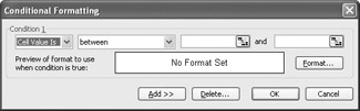
The first list box lets you choose whether you want the condition that follows to look at the cell s contents or the formula in the cell. In almost every circumstance, you will use the contents of the cell as the test value for the condition.

Tip	The only time you would want to set a formula as the basis for the condition would be to format a certain result, such as a grand total, the same way every time it appeared in a worksheet.

The second list box in the Conditional Formatting dialog box lets you select the comparison to be made. Depending on the comparison you choose, the dialog box will have either one or two boxes in which you enter values to be used in the comparison. The default comparison between requires two values, whereas comparisons such as less than require one.

After you have created a condition, you need to define the format to be applied to data that meets that condition. You do that in the Format Cells dialog box. From within this dialog box, you can set the characteristics of the text used to print the value in the cell. When you re done, a preview of the format you defined appears in the Conditional Formatting dialog box.

You re not limited to creating one condition per cell. If you like, you can create additional conditions by clicking the Add button in the Conditional Formatting dialog box. When you click the Add button, a second condition section appears.

Important

Excel doesn t check to make sure your conditions are logically consistent, so you need to be sure you enter your conditions correctly.

Excel evaluates the conditions in the order you entered them in the Conditiona Formatting dialog box and, upon finding a condition the data meets, stops its comparisons. For example, suppose Catherine wanted to visually separate the credit limits of The Garden Company s customers into two different categories: those with limits under $1,500 and those with limits from $1,500 to $2,500. She could display her customers credit limits with a conditional format using the conditions in the following graphic.

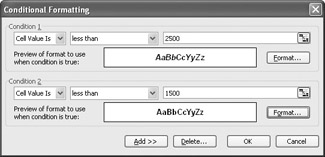
In this case, Excel would compare the value 1250 with the first condition, < 2500 , and assign that formatting to the cell containing the value. That the second condition, < 1500 , is closer is irrelevant ”once Excel finds a condition the data meets, it stops comparing.

Tip	You should always enter the most restrictive condition first. In the preceding example, setting the first condition to < 1500 and the second to < 2500 would resultin the proper format.

In this exercise, you create a series of conditional formats to change the appearance of data in worksheet cells displaying the credit limit of The Garden Company s customers.

USE the Conditional.xls document in the practice file folder for this topic. This practice file is located in the My Documents\Microsoft Press\Office 2003 SBS\ChangingDocAppeance folder, and can also be accessed by clicking Start/All Programs/Microsoft Press/Microsoft Office System 2003 Step by Step .

OPEN the Conditional.xls document.

If necessary, click cell K4.
On the Format menu, click Conditional Formatting .

The Conditional Formatting dialog box appears.
In the second list box, click the down arrow and then, from the list that appears, click between .

The word between appears in the second list box.
In the first argument box, type 1000 .
In the second argument box, type 2000 .
Click the Format button.

The Format Cells dialog box appears.
If necessary, click the Font tab.

The Font tab page appears.
In the Color box, click the down arrow and then, from the color palette that appears, click the blue square.

The color palette disappears, and the text in the Preview pane changes to blue.
Click OK .

The Format Cells dialog box disappears.
Click the Add button.

The Condition 2 section of the dialog box appears.
In the second list box, click the down arrow and then, from the list that appears, click between .

The word between appears in the second list box.
In the first argument box, type 2000 .
In the second argument box, type 2500 .
Click the Format button.

The Format Cells dialog box appears.
In the Color box, click the down arrow and then, from the color palette that appears, click the green square.

The color palette disappears, and the text in the Preview pane changes to green.
Click OK .

The Format Cells dialog box disappears.
Click OK .

The Conditional Formatting dialog box disappears.
In cell K4, click the fill handle, and drag it to cell K6.

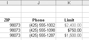
The contents of cells K5 and K6 change to $2,400.00 , and the Auto Fill Options button appears.
Click the Auto Fill Options button, and from the list that appears, click Fill Formatting Only .

The contents of cells K5 and K6 revert to their previous values, and Excel applies the conditional formats to the selected cells.
On the Standard toolbar, click the Save toolbar button to save your changes.

CLOSE the Conditional.xls document.