Manipulating List Data
| Related tasks you can do in Excel 2007 include choosing rows at random from a list and displaying the unique values in a column in the worksheet (not in the down arrow list, which you can't normally work with). Generating a list of unique values in a column can give you important information, such as from which states you have customers or which categories of products sold in an hour. Selecting rows randomly is useful for selecting customers to receive a special offer, deciding which days of the month to audit, or picking prize winners at an employee party. To choose rows, you can use the RAND function, which generates a random value between 0 and 1 and compares it with a test value included in the statement. A statement that returns a TRUE value 30 percent of the time would be RAND()<=30%; that is, whenever the random value was between 0 and .3, the result would be TRUE. You could use this statement to select each row in a list with a probability of 30 percent. A formula that displayed True when the value was equal to or less than 30 percent, and False otherwise, would be =IF(RAND()<=0.3,"True","False"). Tip Because the RAND function is a volatile function (it recalculates its results every time you update the worksheet), you should copy the cells that contain the RAND function in a formula. Then, on the Home tab of the user interface, in the Clipboard group, click the Paste button down arrow and select Paste Values to replace the formula with its current result. Excel 2007 has a new function, RANDBETWEEN, which enables you to generate a random value within a defined range. For example, the formula =RANDBETWEEN(1,100) would generate a random value from 1 to 100, inclusive. The ability to focus on the data that's most vital to your current needs is important, but there are a few limitations. One limitation is that any formulas you create using the SUM and AVERAGE functions don't change their calculations if some of the rows used in the formula are hidden by the filter. Excel 2007 provides two ways to find the total of a group of filtered cells. The first method is to use AutoCalculate. To use AutoCalculate, you select the cells you want to find the total for. When you do, Excel 2007 displays the average of values in the cells, the sum of the values in the cells, and the number of visible cells (count) in the selection. You'll find the display on the status bar at the lower edge of the Excel 2007 window. When you use AutoCalculate, you aren't limited to finding the sum of the selected cells. To display the other functions you can use, right-click the AutoCalculate pane and select the function you want from the shortcut menu that appears. AutoCalculate is great for finding a quick total or average for filtered cells, but it doesn't make the result available in the worksheet. Formulas such as =SUM(C3:C26) always consider every cell in the range, regardless of whether a cell's row is hidden by a filter, so you need to create a formula using the SUBTOTAL function. The SUBTOTAL function, which enables you to summarize only the visible cells in a range, has this syntax: SUBTOTAL(function_num, ref1, ref2, ...). The function_num argument holds the number of the operation you want to use to summarize your data. The ref1, ref2, and further arguments represent up to 29 ranges to include in the calculation. For example, the formula =SUBTOTAL(9, C3:C26, E3:E26, G3:G26) would find the sum of all values in the ranges C3:C26, E3:E26, and G3:G26. Caution Be sure to place your SUBTOTAL formula on a row that is even with or above the headers in the range you're filtering. If you don't, your filter might hide the formula's result! The following table lists the summary operations available to you in a SUBTOTAL formula. The function numbers in the first column include all values in the summary; the function numbers in the second column summarize only those values that are visible within the worksheet.
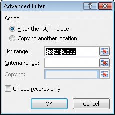
Note Excel 2007 displays the available summary operations as part of the Formula AutoComplete functionality, so you don't need to remember the operation codes or look them up in the Help system. If you want to find a list of the unique values in a data list row, click any cell in the data list, display the Data tab of the user interface, and then in the Sort & Filter group, click Advanced to display the Advanced Filter dialog box. In the List Range field, type the reference of the cell range you want to examine for unique values, select the Unique records only check box, and then click OK to have Excel 2007 display the first occurrence of each value in the column. Important Excel 2007 treats the first cell in the data range as a header cell, so it doesn't consider the cell as it builds the list of unique values. Be sure to include the header cell in your data range! In this exercise, you will select random rows from a list of exceptions to identify package delivery misadventures to investigate, create a SUBTOTAL formula to summarize the visible cells in a filtered data list, and find the unique values in one column of a data list.
USE the ForFollowUp workbook in the practice file folder for this topic. This practice file is located in the My Documents\Microsoft Press\Excel SBS\Focusing folder. OPEN the ForFollowUp workbook.
CLOSE the ForFollowUp workbook. |


EAN: 2147483647
Pages: 143