9.2 Basic notation

---

9.2 Basic notation

Petri nets represent computer systems by providing a means to abstract the basic elements of the system and its informational flow using only four fundamental components. These four Petri net modeling components are place, transition, arc, and token. Places are represented graphically as a circle, transitions as a bar, arcs as directed line segments, and tokens as dots (Figure 9.1). Places are used to represent possible system components and their state. For example, a disk drive could be represented using a place, as could a program or other resource. Transitions are used to describe events that may result in different system states. For example, the action of reading an item from a disk drive or the action of writing an item to a disk drive could be modeled as separate transitions. Arcs represent the relationships that exist between the transitions and places. For example, disk read requests may be put in one place, and that place may be connected to the transition, "removing an item from a disk," thus indicating that this place is related to the transition. You can think of the arc as providing a path for the activation of a transition. Finally, tokens are used to define the state of the Petri net. Tokens in the basic Petri net model are nondescriptive markers, which are stored in places and are used in defining Petri net marking.

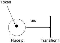
Figure 9.1: Basic Petri net components.

The marking of a Petri net place by the placement of a token can be viewed as the statement of the condition of the place. For example, Figure 9.2 illustrates a simple Petri net with only one place and one transition. The place is connected to the transition by an arc, and the transition is likewise connected to the place by a second arc. The former arc is an input arc, while the latter arc is an output arc. The placement of a token represents the active marking of the Petri net state. The Petri net shown in Figure 9.2 represents a net that will continue to cycle forever.

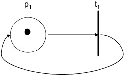
Figure 9.2: Example perpetual motion Petri net.

Petri nets are described both graphically and using set notation. As described previously, a Petri net is composed of places (P), transitions (T), arcs (consisting of input functions, I, and output functions, O), and tokens, which form the marking of the net (MP). Using this notation, we can describe a Petri net as a five tuple, M = (P,T,I,O, MP), where P represents a set of places, P = {p₁, p₂, ... ,p_n}, with one place for each circle in the Petri net graph; T represents a set of transitions, T = {t₁, t₂, ... ,t_m}, with one for each bar in the Petri net graph; I represents a bag of sets (bags is a generalization allowing for duplicates) of input functions for all transitions, I = {I_t1,I_t2, ... ,I_tm}, mapping places to transitions;, O represents a bag of sets of output functions for all transitions, O = {O_t1,O_t2, ... ,O_tm}, mapping transitions to places; and MP represents the marking of places with tokens. The initial marking is referred to as MP₀. MP₀ is represented as an ordered tuple of magnitude n, where n represents the number of places in our Petri net. Each place will have either no tokens or some integer number of tokens. For example, the Petri net graph depicted in Figure 9.3 can be described using the previous notation as:

(9.1)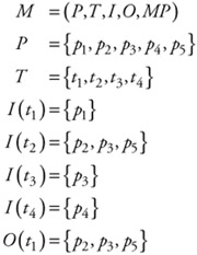 

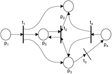
Figure 9.3: Petri net example.

The graphical notation depicts Petri nets as a directed bipartite graph. The graph, G, is described as a two tuple, G = (V,A), where V represents a set of vertices, V = {v₁, v₂, v_3, ... ,v_s}; and A represents a bag of directed arcs, A = {a₁, a₂, a₃, ... ,a_i}. An arc, which is an element of A, is composed of a tuple with two vertices, a_i = (v_j,v_k), where v_j,v_k ∈ V. The set of vertices of the graph can be partitioned into two disjoint sets, P and T, where these sets have the properties V = P ⋃ T and P ⋂ T = 0. In addition, for an arc a_i ∈ A, if a_i = (v_j,v_k), then either v_j ∈ P and v_k ∈ T or vice versa. That is, the two ends of the arc cannot be drawn from the same set; if v_j ∈ P, then v_k ∈ T and cannot be an element of P.

A Petri net model, as with many mathematical models, has a dual. The dual of a Petri net is defined as a Petri net where transitions are changed to places and places are changed to transitions. (See Figure 9.4.) The input and output functions are changed in that the inputs defined for the transition now represent inputs to places. Since this is not possible, the inputs become output functions and output functions become input functions.

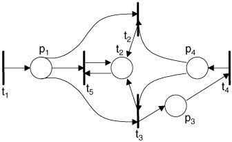
Figure 9.4: Dual of Petri Net from Figure 9.3.

A Petri net can also have an inverse defined for it. The inverse of a Petri net keeps all places and transitions the same and switches the input functions with the output functions (Figure 9.5).

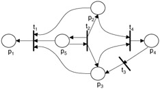
Figure 9.5: Inverse of Petri Net from Figure 9.3.

Petri nets are defined also as multigraphs, since a place can represent multiple inputs and/or outputs from or to a transition. This implies that there could be several arcs between a single place and a transition. We could model these as single arcs but that could become cumbersome as the number of arcs grows. A better way to model multiple arcs is either to represent the multiple arcs as a thick arc with the number of representative arcs embedded inside (Figure 9.6), or as a bold arc with a number attached to it as a label (Figure 9.7).

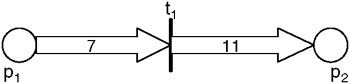
Figure 9.6: Multipath arc.

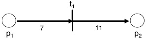
Figure 9.7: Multipath arc as bold line.

Petri nets have a state. This state is defined by the cardinality of tokens and their distribution throughout the places in the Petri net. This marking can be represented as a function, μ, defined over each place, p, and results in a value, N, from the set of counting integers 0, 1, ... ,∞:

(9.2) 

The marking, μ, can also be defined as an n vector. The vector μ provides token information for each place, p_i, in a Petri net. The token information represents the number of tokens in the particular place (number of tokens in place, p_i, is μ_i):

(9.3) 

where

n = |P| and each μ_i ∈ N,i = 0,...,n

Place markings represented as a function and place markings represented as a vector are related by μ(p_i) = μ_i. The markings at a specific point in time represent the state of the Petri net at that time. A marked Petri net, M = (C, μ), is represented as a Petri net structure, M = (P, T, I, O) and its marking: MP or μ. This is also typically represented as M = (P, T, I, O, μ). The marking μ changes as the Petri net changes state and is therefore typically represented with a subscript t. Therefore, the true representation is:

(9.4) 

where represents the state of the Petri net at time t, where t is drawn from the set of nonnegative integer values.

The marking of a Petri net is specified by placing tokens, which are represented as dots in the graphical notation (Figure 9.8) in the places. The marking for the Petri net shown in Figure 9.8 represented as a vector would be μ_t = (1,2,0,0,1). If we assume this is the initial marking of this Petri net, then the definition becomes μ₀ = (1,2,0,0,1), since this would be the 0th state this Petri net has visited. The number of tokens that may be assigned to a place is unbounded (though in later refined models we will see this can be limited). The set of all possible markings for a Petri net with n places is simply the set of all n vectors, Nⁿ, where N represents all possible states and n the number of places.

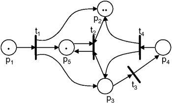
Figure 9.8: Marked Petri net.

---