4.2
4.2 "RT UML" ProfileThe so-called RT UML Profile (RTP), more formally known as the UML Profile for Schedulability, Performance, and Time, was submitted in response to a Request for Proposal (RFP) written up by the Real-Time Analysis and Design Working Group (RTAD) of the OMG, of which I am a cochair, as well as a co-submitter of the profile. The purpose of the profile was to define a common, standard way in which timeliness and related properties could be specified, and the primary benefit of the profile was seen to be the ability to exchange quantitative properties of models among tools. Specifically, we wanted to be able to define a standard way for users to annotate their models with timely information, and then allow performance analysis tools read those models and perform quantitative analysis on them. A consortium of several companies was formed to respond to the RFP. The result was the profile as it was approved and voted to be adopted in 2001. Following the voting, the Finalization Task Force (FTF) was formed to remove defects and resolve outstanding issues. The FTF has completed its work and the profile is now maintained by the Revision Task Force (RTF). The RFP specifically calls for submissions that "define standard paradigms for modeling of time-, schedule- and performance-related aspects of real-time systems." This does not in any way mean that these things cannot be modeled in the UML without this profile. Indeed, the approach the submissions team took was to codify the methods already in use to model time, schedulability, and performance, and then define a standard set of stereotypes and tags. Thus, the tag SApriority allows the user to specify the priority of an active class in a way that a performance analysis tool knows how to interpret. Several guiding principles were adhered to during the creation of the proposal. First and foremost, the existing UML cannot be changed in a profile. We also did not want to limit how users might want to model their systems. We all felt that there is no one right way to model a system, and we wanted to allow the users freedom to choose the modeling approach that best suited their needs. We did not want to require the user to understand the detailed mathematics of the analytic methods to be applied, and we wanted the approach used to be scalable. By scalable, we meant that for a simple analysis, adding the quantitative information should be simple and easy, but for more complex models it was all right to require additional effort. In general, if the analysis or the model were 10 times more complex, then one might reasonably expect 10 times the effort in entering the information. We wanted to provide good support for the common analytical methods such as rate monotonic analysis (RMA) and deadline monotonic analysis (DMA), but we did not want to limit the profile to only such methods. We did not want to specify the analytic methods at all, but concentrate instead on how to annotate user models so that such analysis could easily be done. And finally, we wanted to support the notion that analytic tools could synthesize models and modify the user models to improve performance or schedulability, if appropriate. Figure 4-4 shows the use cases for the profile.[2] The analysis method providers are actors[3] that define the mathematical techniques for analysis and provide tools and models to execute the analysis of user models. The infrastructure providers are actors that provide infrastructures, such as real-time operating systems, distribution middleware such as CORBA ORBs, or other kinds of frameworks or libraries that might be incorporated into user systems. These use cases are important because the performance of these infrastructures can greatly affect the performance of the overall system. If such an infrastructure provider supplies a quantitative model of their infrastructure, this would allow the modeler to better analyze their system. Finally we have the modelers (you guys) that build user models. The Modelers actor represents the people constructing models and wanting to annotate and analyze them. It is the use cases associated with this actor on which I will focus.
Figure 4-4. RT UML Profile Use Cases
The Modeler use cases are used to create the user models, to perform the quantitative analysis on these models, and to implement the analyzed models. The expected usage paradigm for the profile is shown in Figure 4-5. Figure 4-5. Usage Paradigm for the RT Profile
In this figure, the user enters the model into a UML modeling tool, such as Rhapsody from I-Logix, as well as entering the quality of service properties of the elements. A modeling analysis tool, such as Rapid RMA from Tri-Pacific Corporation, inputs the model (most likely via XMI), converts it as necessary into a quantitative model appropriate for the analysis, and applies the mathematical techniques used to analyze the model. Once the analysis is complete, the modeling analysis tool updates the user model perhaps just to mark it as schedulable or perhaps to reorder task priorities to improve performance. Once the model is adequate and validated, the application system is generated from the updated UML model. Because the profile is quite large it is divided into subprofiles for improved understandability and usage. Figure 4-6 shows the organization of the profile. It is possible, for example, that some user might want to use one or a smaller number of parts of the profile but not other parts. By segmenting the profile into subprofile packages, the user isn't burdened with all of aspects of the entire profile unless he or she actually needs them. Figure 4-6. RT UML Profile Organization
The three primary packages of the profile are shown in Figure 4-6. The general resource modeling framework contains the basic concepts of real-time systems and will generally be used by all systems using the framework. This package is subdivided into three smaller subprofiles: RT Resource Modeling, RT Concurrency, and RT Time Modeling. The first of these defines what is meant by a resource a fundamental concept in real-time systems. The second of these defines a more detailed concurrency model than we see in the general UML metamodel. The last specifies the important aspects of time for real-time systems, time, durations, and time sources, such as timers and clocks. The second main package of the profile is called analysis models. In this package, we provide subpackages for different kinds of analytic methods. The Schedulability Analysis (SA) package defines the stereotypes, tags, and constraints for common forms of schedulability analysis. Likewise, the Performance Analysis (PA) package does the same thing for common performance analysis methods. These packages use the concepts defined in the resource, concurrency, and time subprofiles mentioned earlier. The RSA profile specializes the SA profile. As new analytic methods are added, it is anticipated that they would be added as subprofiles in the analysis models package. The last primary package is the infrastructure package. In this package, infrastructure models are added. The RFP specifically called for a real-time CORBA infrastructure model, but it is anticipated that other infrastructure vendors would add their own packages here if they wish to support the profile. In the specification of the profile, each of these packages supplies a conceptual metamodel modeling the fundamental concepts of the specific domain, followed by a set of stereotypes and their associated tagged values and constraints. We will discuss each of these subprofiles in turn and finally provide a more complete example of using the overall profile to provide a user model ready for schedulability analysis. To aid in understanding and tracking down where tags and stereotypes are defined, each tag or stereotype is preceded with a code identifying which subprofile defined the item. Thus, things beginning with "GRM" are defined in the general resource model subprofile, things beginning with PA are to be found in the performance analysis subprofile, and so on. Because UML is undergoing a major internal reorganization as a result of the UML 2.0 effort, the RTP will need to undergo a similar level of revision to make it consistent with the new UML standard. The RTAD as a group has decided (rightly, I believe) that this cannot be done within the confines of the Revision Task Force (RTF) that maintains the profile but will require a new request for proposal (RFP) with new submissions. As of this writing, the new RFP is scheduled to be written in the coming months. 4.2.1 General Resource Model SubprofileAs you might guess, the most important concepts in the GRM subprofile are resource and quality of service. A resource is defined to be a model element with finite properties, such as capacity, time, availability, and safety. A quality of service is a quantitative specification of a limitation on one or more services offered by a resource. The general resource model is built on a classic client-server model. The client requests services to be executed by the server. This service request is called a resource usage and may be accompanied by one more qualities of service (QoS) parameters. QoS parameters come in two flavors offered and required. The client may require some performance QoS from the service during the execution of the service, while the server may provide a QoS parameter. If the offered QoS is at least as good as required, then the QoS parameters are said to be consistent. Figure 4-7 shows this relation schematically. Figure 4-7. Client-Server Basis of the GRM
The basic domain model of resources is shown in Figure 4-8 and the model for static resource usage is shown in Figure 4-9. We see that a descriptor "types" an instance. These classes are subclassed so that a resource (a kind of descriptor) likewise types a ResourceInstance. Resources provide ResourceServices (which type corresponding Resource ServiceInstances), each of which can have an associated quality of service characteristic (and corresponding QoS values on the instance side). This strong separation of specifications and instances allows us to perform either static analysis on the specifications or dynamic analysis on the instances of those specifications. Figure 4-8. Core Resource Model
Figure 4-9. Static Resource Usage Model
An important basis for dynamic models, the causality loop relates the notion of an event occurrence with the execution of a scenario. An event describes a change in state and may be (among others) a stimulus generation or a stimulus reception. A stimulus, from the UML specification, is an instance of communication between objects. This causality loop is shown in Figure 4-10. In it, we see that a scenario associates with a set on instances that receive stimuli. Each stimulus is created by a stimulus generation and results in a stimulus reception. Figure 4-10. Causality Loop
The dynamic resource usage model is used to analyze more complex situations than the much simpler static resource usage model. The static model assumes that properties can be assigned to types and the details of the scenarios need not be characterized. In the dynamic usage model, the internal instances of the executing scenarios are given precise QoS values for analysis. We see in Figure 4-11 that a scenario is composed to an ordered set of ActionExecutions, each of which can have required QoS values. The scenario can also have one or more ResourceServiceInstances, each of which can have an offered QoS value. The ResourceServiceInstances belong to ResourceInstances used in the scenario. Tables 4-1 to 4-6 list the stereotypes defined in this subprofile, along with the applicable metaclasses, tags, and descriptions. Figure 4-11. Dynamic Resource Usage Model
4.2.2 Time Modeling SubprofileThe time modeling subprofile specifies the stereotypes and tags for modeling time and related concepts. These are detailed in Table 4-3.
Tagged values hold values that are taken from its type. TimeValues can be expressed in a number of forms:
Arrival patterns are specified with the RTArrivalPattern tag. There are several kinds: bounded, bursty, irregular, periodic, and unbounded. Formally, the syntax is RTArrivalPattern ::= <bounded-string> | <bursty- string> | <irregular-string> | <periodic-string> | <unbounded-string> bounded-string ::= " 'bounded' ," <time-value> "," <time-value> <bursty-string> ::= " 'bursty' ," <time-value> "," <integer> <irregular-string> ::= " 'irregular' ," <time-value> [ '," <time-value> ]* <periodic-string> ::= " 'periodic' ," <time-value> [ "," <time-value>] <unbounded-string> ::= " 'unbounded' ," <PDF-string> Bound arrival patterns are specified with the keyword bounded, followed by a lower and upper bound, as in "bounded, (0, 'ms'), (15, 'ms')." A bursty arrival pattern means that the arrival of events is correlated in time, that is, the arrival of one event makes it more likely that another event will arrive soon after. Bursty arrival patterns are specified with the bursty key word followed by a time value (indicating the burst interval) and an integer value (indicating the maximum number of events in that interval, as in "bursty, (20, 'ms'), 100)." An irregular arrival pattern describes a series of arrival times. It is specified using the keyword irregular, followed by a list of time values, as in "irregular, (10, 'ms'), (15, 'ms'), (5, 'ms')." The asterisk (*) in the grammar means that the term can be repeated an arbitrarily number of times. Periodic arrival patterns are very common. They are indicated with the keyword period and a time value indicating the period. The period value may optionally be followed by another time value that indicates the maximal deviation from the period (sometimes called jitter), as in "periodic, (100, 'ms), (500, 'us')." Finally, an unbounded arrival pattern is one in which the arrival times are drawn as a renewal process from an underlying probability density function, as described below. An example would be "unbounded, normal (100, 'ms'), (15, 'ms')" to specify a normal (Gaussian) distribution with a mean of 100 ms and a standard deviation of 15 ms. The time subprofile identifies the most common probability density functions (PDFs) used with event time distributions Bernoulli, binominal, exponential, gamma, histogram, normal, Poisson, and uniform. Each of these has one or more parameters qualifying the mathematical properties of the distribution. Bernoulli distribution has a single real parameter specifying the probability (in the range of 0 to 1). Binomial distributions have two parameters, a real (the probability) and an integer (the number of trials). Exponential distributions have a single real parameter, the mean, as in "exponential 100." Gamma distributions have two parameters; the first is an integer k, and the mean from the formula in Equation 4-1. Equation 4-1 Gamma Distribution
A histogram distribution is a set of real number pairs, followed by a single real number. Each number pair indicates the start of an interval and the probability of occurrence within that interval. The last single number defines the ending point for the last interval, as in "histogram, 10, 0.10, 20, 0.50, 30, 0.30, 40, 0.1, 50." A normal distribution is characterized by a mean and standard deviation, as in "normal, 90.5, 8.5." A Poisson distribution has a mean, as in "poisson, 80.5." Lastly, a uniform distribution is characterized by a starting and ending points, as in "uniform 50.0, 150.0." Timing information can be applied to action executions using a set of defined "timing marks," including
These timing marks are used in timing expressions captured in constraints applied against the actions or stimuli, as in
which specifies that the time that a stimulus is received until the initiated action completes is less than 10 ms. Such timing specifications are often made on sequence diagrams, such as that in Figure 4-12. We see some of the messages stereotyped as «RTstimulus» and the actions stereotyped as «RTaction». Timing information is added as tags associated with the stereotypes. In addition, there are some "anonymous timing marks" that allow the annotation of the progress of time during the execution of the scenario. Figure 4-12. Timing Marks
4.2.3 Concurrency Modeling SubprofileThe concurrency subprofile refines the core UML's somewhat vague notions of concurrency. The domain model for the profile's concurrency subprofile is shown in Figure 4-13. The most central concept is that of ConcurrentUnit. A ConcurrentUnit is a kind of ActiveResource, which in turn is a kind of ResourceInstance, a domain concept discussed in Section 4.2.1. An ActiveResource is a resource instance that is able to generate its own stimuli concurrently, that is, independent from other activities. A ConcurrentUnit runs a main scenario and may have one or more StimuliQueues. Because it is a subclass of ResourceInstance, it may also own (via composition) an unbounded number of ResourceServiceInstances (instances of services provided by resources). This is what most closely corresponds to the notions of thread, task, and process found in the operating systems literature. Figure 4-13. Concurrency Subprofile Domain Model
ConcurrentUnits then have a main() operation that invokes the main scenario, which in turn is composed of a set of ActionExecutions and associates with one or more resource service instances. These resource service instances may be either deferred or immediate, and if immediate, they may be either local or remote. An immediate service instance handles incoming requests immediately, spawning new threads to do so if required (local threading) or assumes an existing thread will handle it (the remote threading). When a service instance is deferred, the request or stimulus waits until the receiving server is ready to process it. The ConcurrentUnits may collaborate by sending stimuli to each other this is done via the execution of either synchronous or asynchronous message actions. This domain model is cast into the UML standard as a set of stereotypes and tags, as shown in Tables 4-5 and 4-6. The scenario shown in Figure 4-14 illustrates how the concurrency subprofile tags can be used to indicate relevant quality of service properties. The Atrial Timer and the AtrialModel instances are both active and own their own thread of execution ("ConcurrentUnit," in the profile's parlance). In addition, the Atrial Timer is also an «RTtimer» stereotype. Various messages are stereotyped to allow the appropriate tags to be attached to the message to specify their qualities of service. For example, the toInhibiting message is stereotyped to be a «RTevent» with the RTat tag specified: { RTat = (0, 'ms') } . The set() operation that sets the value and starts the timer is stereotyped to be a «RTstart» kind. Some of the action executions are stereotyped to be either «CRSynch» or «CRAsynch» depending on whether they execute in the thread of the caller («CRSynch») or not («CRAsynch»). Some are also stereotyped to be «RTAction» so that the tag RTDuration can specify the execution time QoS for the action. Figure 4-14. Concurrency Subprofile Stereotypes Example
4.2.4 Schedulability Modeling SubprofileThe previous subprofiles, the general resource model, time, and concurrency subprofiles, do provide useful stereotypes and tags for the specification of important qualities of service, but the schedulability subprofile is where the concepts come together for the most common types of schedulability analysis. The core domain model for the schedulability subprofile is shown in Figure 4-15. This domain model connects to the other domain models in that many of the domain classes are subclasses of classes in the previous subprofiles. For example, SAction is a subclass of Timed Action (from the TimedEvents package in the time subprofile), Trigger is a subclass of UsageDemand (from the ResourceUsageModel of the general resource model subprofile), RealTimeSituation is a subclass of AnalysisContext (from the ResourceUsageModel of the general resource model subprofile), an ExecutionEngine is a subtype of ActiveResource, Processor, and ProtectedResource (all from the ResourceTypes package of the general resource model subprofile), an SResource is a subclass of ProtectedResource (ibid), and SchedulableResource is a subclass of both SResource and ActiveResource. Figure 4-15. Schedulability Domain Model
An SAction, or schedulable action, may contain nested actions. The QoS properties of an SAction may be derived, if necessary, from the QoS properties of its subordinate parts. SActions have a large number of tags that can be used for schedulability analysis, such as SApriority, SAblocking, SAworstCase (worst-case completion time), and so on, as well as those inherited from its superclass TimedAction. These actions engine may be a CPU, operating system, or virtual machine running the scheduling job. A scheduling job is associated with a trigger that starts it off and a response a sequence of actions that is separately schedulable on an execution engine. A response is a subclass of SAction but adds a few more QoS aspects, such as utilization, slack time, spare capacity, and how many instances of the response may overlap their execution in the case of missed deadlines. An SResource is a kind of protected resource that is accessed during the execution of a scheduling job. Because it may be shared among concurrently executing actions, it must be protected with a mutual exclusion lock such as a semaphore or by a policy that prevents simultaneous access. Examples of an SResource are a shared queue or A/D converter. A SchedulableResource is a kind of SResource that is used to execute one or a set of actions. This domain class represents a task, thread, or process in the OS world. These domain concepts are mapped into the stereotypes and tagged values identified in Tables 4-7 through 4-12.
All this probably seems confusing, more from the plethora of stereotypes and tags than from their inherent complexity. In actual fact, you will most likely use a small subset of the stereotypes and tags in any given analysis of schedulability. Different kinds of analysis will tend to use different stereotypes and tags. For example, look at the model in Figure 4-16. It contains five active objects, each of which owns a thread. The properties of these threads, such as the occurrence pattern ("periodic"), the period, worst-case execution time, and so on are all provided as tagged values in the constraints. In this case, the higher the value of the priority, the lower the priority; in the model; the classes with priority 100 are the lowest priority threads. Note that the lowest priority threads have no blocking term because, by definition, they cannot be blocked, only preempted. There are also three resources (waveform queues), different instances of the same class, Waveform. To perform schedulability analysis on this model is straightforward. Figure 4-16. Schedulability Subprofile Example (Global RMA)
First, remember the global RMA analysis inequality shown in Equation 4-2. Equation 4-2 Rate Monotonic Analysis with Blocking
in which Cj is the worst-case execution time for task j, Tj is the period of task j, Bj is the blocking time for task j, and n is the number of tasks. Inserting the information from the tags into the inequality, we get Equation 4-3. Equation 4-3 Analysis of Static Model
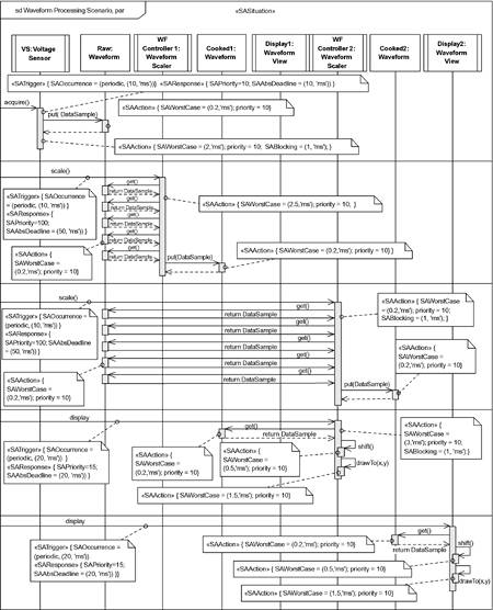
Since the inequality is true, we can guarantee that the system is schedulable; that is, it will always meet its deadlines, regardless of task phasings. More detailed analysis can be done by looking at the sequences of actions rather than merely at the active objects. This is usually done if the global RMA analysis fails, indicating that the system can't be guaranteed (by that analysis) to be schedulable. The global analysis method is often overly strong just because it can't be guaranteed by the method to be schedulable doesn't mean that it isn't. It just means that the analytic method can't guarantee it. However, a more detailed analysis may be able to guarantee it. A more detailed analysis might analyze a specific scenario, or class of scenarios. Such a scenario is shown in Figure 4-17. This sequence diagram uses both the sd and the par operators, so that the interaction subfragments (separated by operand separators) are running concurrently. The scenario is schedulable if it can be demonstrated that all of its concurrent parts can meet their deadlines, including any preemption due to the execution of peer concurrent interactions. Figure 4-17. Schedulability Subprofile Example (Scenario Analysis)
In this scenario, the timing and scheduling information is provided in a more detailed view from which the global summary may be constructed. For example, in the first parallel interaction fragment, the acquire() method is stereotyped to be both an SAtrigger (so it can have an occurrence pattern and period) and an SAresponse (so it can have a priority and a deadline). The timing properties of each of the call actions are defined. Since priority inheritance is used to limit priority inversion, an action may be blocked by, at most, a single lower- priority action. The blocking time for the overall sequential thread of execution is the largest blocking term for any of its subactions. 4.2.5 Performance Modeling SubprofileThe performance analysis (PA) subprofile is concerned with annotating a model for computation of system performance. Specifically, this profile uses the concepts and tags defined in the resource, concurrency, and time subprofiles to create stereotypes and tags that are useful for adding quantitative measures of performance, so that overall system performance analysis may be performed. Note that is this different from schedulability analysis, which analyzes a system to ensure whether it can meet its schedulability requirements. Performance analysis is inherently instance-based (as opposed to class- or type-based). Scenarios, sequences of steps for which at least the first and last steps are visible, are associated with a workload or a response time. Open workloads are defined by streams of service requests that have stochastically characterized arrival patterns, such as from a Poisson or Gaussian distribution. Closed workloads are defined by a fixed number of users or clients cycling among the clients for service requests. Scenarios, as we have seen, are composed of scenario steps, which are sequences of actions connected by operators such as decision branches, loops, forks, and joins. Scenario steps may themselves be composed of smaller steps. Scenario steps may use resources via resource demands, and most of the interesting parts of performance analysis have to do with how a finite set of resource capabilities are shared among their clients. Resources themselves are modeled as servers. Performance measures are usually modeled in terms of these resources, such as the percentage of resource utilization or the response time of a resource to a client request. Within those broad guidelines, these measures may be worst case, average case, estimated case, or measured case. Performance analysis is normally done either with queuing models or via simulation. Queuing models assume that requests may wait in a FIFO queue until the system is ready to process them. This waiting time is a function of the workload placed on the resources as well as the time (or effort) required by the system to fulfill the request once started. In simple analysis, it may only require the arrival rates of the requests and the response time or system utilization required to respond. More detailed analyses may require distributions of the request occurrences as well. Simulation analysis logically "executes" the system under different loads. A request in process is represented as a logical token and the capacity of the system is the number of such tokens the may be in process at one time. Because of bottlenecks, blocking, and queuing, it is possible to compute the stochastic properties of the system responses. The domain model for performance modeling is shown in Figure 4-18. As discussed earlier, a scenario is associated with a workload, the latter being characterized in terms of a response time and a priority. Scenarios use resources and are composed of scenario steps. Resources may be passive or active processors resources. The elements of this domain model which are subclasses of elements in other profiles are shown with the base elements colored and the packages from whence they are defined are shown using the scope dereference operator "::". Figure 4-18. Performance Domain Model
These domain concepts are used to identify stereotypes of UML elements, and the domain concept attributes are defined as tags in the performance analysis profile. Tables 4-13 through 4-18 give the stereotypes, the applicable UML metaclasses, the associated tags, and a brief description. There are a few special types used in the tag definitions above. Specifically, SchedulingEnumeration, PAperfType, and PAextOpValue. The SchedulingEnumeration type specifies various scheduling policies that may be in use. These are commonly exclusive. The PA profile defines the following types of scheduling policies:
The PAperfValue is a performance value type of the form "(" <source-modifier> "," <type-modifier> "," <time-value> ")" The source modifier is a string that may be any of the following:
The type modifier may be any of the following expressions:
The time value is defined by the specification of RTtimeValue provided in the section of schedulability. For example:
PAestOpValue is a string used to identify an external operation and either the number of repetitions of the operation or a performance time value. The format is of the form "(" <String> "," <integer> | <time-value> ")" where the string names the external operation and the integer specifies the number of times the operation is invoked. The time value is of type PAperValue and specifies a performance property of the external operation. The three figures that follow, Figures 4-19 through 4-21, provide an example model that can be analyzed for performance. Figure 4-19 shows the object structure of the system to be analyzed an engine control system that includes a Doppler sensor for detecting train velocity, an object that holds current speed (and uses a filtering object to smooth out high-frequency artifacts), and an engine controller that uses this information to adjust engine speed plus two views for the train operator, a textual view of the current speed (after smoothing) and a histogram view that shows the recent history of speed. Figure 4-19. Performance Model Example (Structure)
Figure 4-20 shows how these objects are deployed. In this case, there are four distinct processing environments. A low-power acquisition module reads the emitted light after it has been reflected off the train track and computes an instantaneous velocity from this, accounting for angle and at least in a gross way for reflection artifacts. This process runs at a relative rate of 10. Since the reference is the 1MBit bus, this can be considered to be 10MHz. Note the "$Util" in the constraint attached to the processor this is where a performance analysis tool would insert the computed utilization once it has performed the mathematical analysis. Figure 4-20. Performance Model Example (Deployment)
As with all the processors, this computer links to the others over a 1Mbit CAN bus link. The CAN bus uses its 11-bit header (the CAN bus also comes in a 29-bit header variety) to arbitrate message transmission using a "bit dominance" protocol,[6] a priority protocol in which each message header has a different priority.
The controller computer runs the TrainSpeed object and its associated data filter. It runs at the same rate as the acquisition module. The EngineController and Engine objects run on the Engine computer, which also runs at the 10MHz rate. The last computer is much faster, running at 2,000 times the rate of the bus, 2GHz. It runs the display software for showing the current speed (via the SpeedView object) and the histogram of the speed (via the SpeedHistory object). Lastly, Figure 4-21 shows an example of execution. Note that the execution on the different processors is modeled in parallel regions in the sequence diagram (the interaction fragments within the par operator scope), and within each the execution is sequential. Messages are sent among the objects residing on different processors, as you would expect, and the time necessary to construct the message, fragment it (if necessary the CAN bus messages are limited to 8 bytes of data), transmit it, reassemble the message on the target side, do the required computational service, and then repeat the process to return the result is all subsumed within the execution time of the operation. A more detailed view is possible that includes these actions, (construct, fragment, transmit, receive, reconstruct, invoke the desired service, construct the response message, fragment it, transmit it, reassemble it on the client side, extract the required value, and return it to the client object). However, in this example, all those smaller actions are considered to be executed within the context of the invoked service, so that calls to TrainSpeed.getSpeed() are assumed to include all those actions. For an operation invoked across the bus that requires 1 ms to execute, the bus transmission alone (both ways) would require on the something a bit less than 200 us, assuming that a full 8 bytes of data (indicating the object and service to be executed) are sent. There will be a bit more overhead to parse the message and pass it off to the appropriate target object. Thus, the time overhead for using the CAN bus shouldn't be, in general, more than 500 us to 1 ms unless large messages are sent (requiring message fragmentation) or unless the message is of low priority and the bus is busy. This does depend on the application protocol used to send the messages and the efficiency of the upper layers of the protocol stack. Figure 4-21. Performance Model Example (Scenario)
4.2.6 Real-Time CORBA SubprofileThe RFP for the RTP requires that submissions include the ability to analyze real-time CORBA (RT CORBA) models. CORBA stands for Common Request Broker Architecture and is a middleware standard also owned by the Object Management Group. A detailed discussion of CORBA is beyond the scope of this book but a short description is in order. CORBA supports systems distributed across multiple processor environments. The basic design pattern is provided in [4]:
Figure 4-22a. Broker Pattern (Simplified). From [4]
Figure 4-22b. Broker Pattern (Elaborated). From [4].
The domain model for real-time CORBA is shown in Figure 4-23. Note that the RTCorb (Real-Time CORBA Orb) is a processing environment and the domain models contain RTCclients and RTCservers as expected. All the domain concepts are prefaced with RTC, while the profile stereotypes and tags are prefaced with RSA (real-time CORBA schedulability analysis). The following tables show the defined stereotypes. Figure 4-23. Real-Time CORBA Domain Model
An RSAschedulingPolicy is one of the following enumerated values: { 'FIFO', 'RateMonotonic', 'DeadlineMonotonic', 'HKL', 'FixedPriority', 'MinimumLaxityFirst', 'MaximizeAccruedUtility', 'MinimumSlackTime'}. An SAschedulingPolicy is one of the following enumerated values: { 'FIFO', 'PriorityInheritance', 'NoPreemption', 'HighestLockers', 'PriorityCeiling'}.
| ||||||||||||||||||||||||||||||||||||||||||||||||||||||||||||||||||||||||||||||||||||||||||||||||||||||||||||||||||||||||||||||||||||||||||||||||||||||||||||||||||||||||||||||||||||||||||||||||||||||||||||||||||||||||||||||||||||||||||||||||||||||||||||||||||||||||||||||||||||||||||||||||||||||||||||||||||||||||||||||||||||||||||||||||||||||||||||||||||||||||||||||||||||||||||||||||||||||||||||||||||||||||||||||||||||||||||||||||||||||||||||||||||||||||||||||||||||||||||||||||||||||||||||||||||||||||||||||||||||||||||||||||||||||||||||||||||||||||||||||||||||||||||||||||||||||||||||||||||||||||||||||||||||||||||||||||||||||||||||||||||||||||||||||||||||||||||||||||||||||||||||||||||||||||||||||||||||||||||||||||||||||||||||||||||||||||||||||||||||||||||||||||||||||||||||||||
EAN: 2147483647
Pages: 127