Understanding Lookup and Reference Functions
 Lookup and reference functions help you use your own worksheet tables as sources of information to be used elsewhere in formulas. You can use three primary functions to look up information stored in a list or a table or to manipulate references: LOOKUP, VLOOKUP, and HLOOKUP. Some powerful lookup and reference functions in addition to these three are available; we describe many of them in the following sections. You'll find a list of all these functions by clicking the Lookup & Reference button on the Formulas tab on the Ribbon.
Using Selected Lookup and Reference Functions
VLOOKUP and HLOOKUP are nearly identical functions that look up information stored in tables you have constructed. VLOOKUP and HLOOKUP operate in either vertical or horizontal orientation (respectively), but LOOKUP works either way.
When you look up information in a table, you usually use a row index and a column index to locate a particular cell. Excel derives the first index by finding the largest value in the first column or row that is less than or equal to a lookup value you supply and then uses a row number or column number argument as the other index. Make sure the table is sorted by the row or column containing the lookup values.
You can create powerful lookup formulas using add-in tools. (The tools don't actually use any of the lookup functions.) For more information, see "Using the Conditional Sum and Lookup Wizards" on page 478.
These functions take the following forms:
=VLOOKUP(lookup_value, table_array, col_index_num, range_lookup) =HLOOKUP(lookup_value, table_array, row_index_num, range_lookup)
Table 14-1 lists LOOKUP function arguments and their descriptions. The LOOKUP function takes two forms; the first is called the vector form, and the second is called the array form:
=LOOKUP(lookup_value, lookup_vector, result_vector) =LOOKUP(lookup_value, array)
| Argument | Description |
|---|---|
| lookup_value | The value, cell reference, or text (enclosed in quotation marks) that you want to find in a table or a range. |
| table_array | A cell range or name that defines the table in which to look. |
| row_index_num col_index_num | The row or column number of the table from which to select the result, counted relative to the table (not according to the actual row and column numbers). |
| range_lookup | A logical value that determines whether the function matches lookup_value exactly or approximately. Type FALSE to match lookup_value exactly. The default is TRUE, which finds the closest match. |
| lookup_vector | A one-row or one-column range that contains numbers, text, or logical values. |
| result_vector | A one-row or one-column range that must be the same size as lookup_vector. |
| array | A range containing numbers, text, or logical values to compare with lookup_value. |
The difference between the lookup functions is the type of table each function uses: VLOOKUP works only with vertical tables (tables arranged in columns); HLOOKUP works only with horizontal tables (tables arranged in rows). You can use the array form of LOOKUP with either horizontal tables or vertical tables, and you can use the vector form with single rows or columns of data.
The array form of LOOKUP determines whether to search horizontally or vertically based on the shape of the table defined in the array argument. If the table has more columns than rows, LOOKUP searches the first row for lookup_value; if the table has more rows than columns, LOOKUP searches the first column for lookup_value. LOOKUP always returns the last value in the row or column containing the lookup_value argument; or you can specify a row or column number using VLOOKUP or HLOOKUP.
The VLOOKUP and HLOOKUP Functions
For the VLOOKUP and HLOOKUP functions, whether Excel considers a lookup table to be vertical or horizontal depends on where the comparison values (the first index) are located. If the values are in the leftmost column of the table, the table is vertical; if they are in the first row of the table, the table is horizontal. (In contrast, LOOKUP uses the shape of the table to determine whether to use the first row or column as the comparison values.) The comparison values can be numbers or text, but it is essential that they be sorted in ascending order. No comparison value should be used more than once in a table.
The index_num argument (sometimes called the offset) provides the second index and tells the lookup function which column or row of the table to look in for the function's result. The first column or row in the table has an index number of 1; therefore, the index_num argument must be greater than or equal to 1 and must never be greater than the number of rows or columns in the table. For example, if a vertical table is three columns wide, the index number can't be greater than 3. If any value does not meet these rules, the function returns an error value.
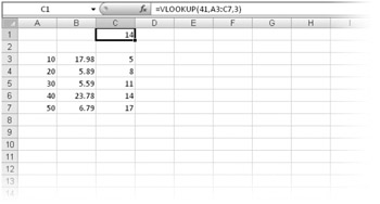
You can use the VLOOKUP function to retrieve information from the table in Figure 14-2.

Figure 14-2: You can use the VLOOKUP function to retrieve information from a vertical table like this one.
On the CD You'll find the ![]() Lookup.xlsx file in the Sample Files section of the companion CD.
Lookup.xlsx file in the Sample Files section of the companion CD.
Remember that these lookup functions usually search for the greatest comparison value that is less than or equal to the lookup value, not for an exact match between the comparison values and the lookup value. If all the comparison values in the first row or column of the table range are greater than the lookup value, the function returns the #N/A error value. If all the comparison values are less than the lookup value, however, the function returns the value that corresponds to the last (largest) comparison value in the table, which might not be what you want. If you require an exact match, type FALSE as the range_lookup argument.
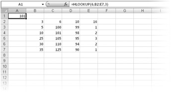
The worksheet in Figure 14-3 shows an example of a horizontal lookup table using the HLOOKUP function.

Figure 14-3: You can use the HLOOKUP function to retrieve information from a horizontal table like this one.
The LOOKUP Function
The LOOKUP function is similar to VLOOKUP and HLOOKUP and follows the same rules, but it is available in two forms, vector and array, whose arguments are described in Table 14-1.
Like HLOOKUP and VLOOKUP, the vector form of LOOKUP searches for the largest comparison value that isn't greater than the lookup value. It then selects the result from the corresponding position in the specified result range. The lookup_vector and result_vector arguments are often adjacent ranges, but they don't have to be when you use LOOKUP. They can be in separate areas of the worksheet, and one range can be horizontal and the other vertical. The only requirement is that they must have the same number of elements.
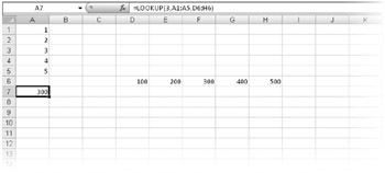
For example, consider the worksheet in Figure 14-4, where the ranges are not parallel. Both the lookup_vector argument, A1:A5, and the result_vector argument, D6:H6, have five elements. The lookup_value argument, 3, matches the entry in the third cell of the lookup_vector argument, making the result of the formula the entry in the third cell of the result range: 300.

Figure 14-4: The vector form of the LOOKUP function can retrieve information from a nonparallel cell range.
The array form of LOOKUP is similar to VLOOKUP and HLOOKUP but works with either a horizontal table or a vertical table, using the dimensions of the table to figure out the location of the comparison values. If the table is taller than it is wide or the table is square, the function treats it as a vertical table and assumes that the comparison values are in the leftmost column. If the table is wider than it is tall, the function views the table as horizontal and assumes that the comparison values are in the first row of the table. The result is always in the last row or column of the specified table; you can't specify column or row numbers.
Because HLOOKUP and VLOOKUP are more predictable and controllable, you'll generally find using them preferable to using LOOKUP.
The ADDRESS Function
The ADDRESS function provides a handy way to build a cell reference using numbers typed into the formula or using values in referenced cells. It takes the arguments (row_ num, column_num, abs_num, a1, sheet_text). For example, the formula =ADDRESS(1, 1, 1, TRUE, "Data Sheet") results in the reference 'Data Sheet'!$A$1.
The CHOOSE Function
You use the CHOOSE function to retrieve an item from a list of values. The function takes the arguments (index_num, value 1, value 2,...) and can include up to 254 values. The index_num argument is the position in the list you want to return; it must be positive and can't exceed the number of elements in the list. The function returns the value of the element in the list that occupies the position indicated by index_num. For example, the function =CHOOSE(2, 6, 1, 8, 9, 3) returns the value 1, because 1 is the second item in the list. (The index_num value isn't counted as part of the list.) You can use individual cell references for the list, but you can't specify ranges. You might be tempted to create a function, such as =CHOOSE(A10, C1:C5), to take the place of the longer function in the preceding example. If you do, however, the result is a #VALUE! error value.
The MATCH Function
The MATCH function is closely related to the CHOOSE function. However, whereas CHOOSE returns the item that occupies the position in a list specified by the index_num argument, MATCH returns the position of the item in the list that most closely matches a lookup value.
| Note | You can create powerful lookup formulas using add-in tools that use the MATCH and INDEX functions. See "Using the Conditional Sum and Lookup Wizards" on page 478. |
This function takes the arguments (lookup_value, lookup_array, match_type), where lookup_value and the items in the lookup_array can be numeric values or text strings, and match_type defines the rules for the search, as shown in Table 14-2.
| match_type | Description |
|---|---|
| 1 (or omitted) | Finds the largest value in the specified range (which must be sorted in ascending order) that is less than or equal to lookup_value. If no items in the range meet these criteria, the function returns #N/A. |
| 0 | Finds the first value in the specified range (no sorting necessary) that is equal to lookup_value. If no items in the range match, the function returns #N/A. |
| -1 | Finds the smallest value in the specified range (which must be sorted in descending order) that is greater than or equal to lookup_value. If no items in the range meet these criteria, the function returns #N/A. |
When you use MATCH to locate text strings, you should specify a match_type argument of 0 (an exact match). You can then use the wildcards * and ? in the lookup_value argument.
The INDEX Function
The INDEX function has two forms: an array form, which returns a value, and a reference form, which returns a cell reference. The forms of these functions are as follows:
=INDEX(array, row_num, column_num) =INDEX(reference, row_num, column_num, area_num)
The array form works only with an array argument; it returns the value of the result, not the cell reference. The result is the value at the position in array indicated by row_num and column_num. For example, the formula
=INDEX({10,20,30;40,50,60}, 1, 2) returns the value 20, because 20 is the value in the cell in the second column and first row of the array.
| Note | Each form of the INDEX function offers an advantageous feature. Using the reference form of the function, you can use multiple, nonadjacent areas of the worksheet as the reference lookup range. Using the array form of the function, you can get a range of cells, rather than a single cell, as a result. |
The reference form returns a cell address instead of a value and is useful when you want to perform operations on a cell (such as changing the cell width), rather than on its value. This function can be confusing, however, because if an INDEX function is nested in another function, that function can use the value in the cell whose address is returned by INDEX. Furthermore, the reference form of INDEX doesn't display its result as an address; it displays the value(s) at that cell address. Remember that the result is an address, even if it doesn't look like one.
Here are a few guidelines to keep in mind when using the INDEX function:
-
If you type 0 as the row_num or column_num argument, INDEX returns a reference for the entire row or column, respectively.
-
The reference argument can be one or more ranges, which are called areas. Each area must be rectangular and can contain numbers, text, or formulas. If the areas are not adjacent, you must enclose the reference argument in parentheses.
-
You need the area_num argument only if you include more than one area in reference. The area_num argument identifies the area to which the row_num and column_num arguments will be applied. The first area specified in reference is designated area 1, the second area 2, and so on.
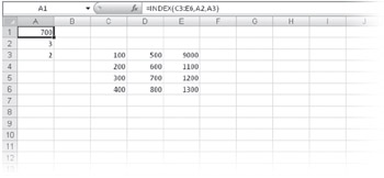
Let's consider some examples to see how all this works. Figure 14-5 shows an example of an INDEX function. The formula in cell A1 uses the row coordinate in cell A2 and the column coordinate in cell A3 to return the contents of the cell in the third row and second column of the specified range.

Figure 14-5: Use the INDEX function to retrieve the address or value in a cell where information is located.
The following example is a bit trickier: Using the same worksheet in Figure 14-5, the formula =INDEX(C3:E6, 0, 2) displays the #VAEUE! error value because the row_num argument of 0 returns a reference to the entire column specified by the column_num argument of 2, or the range D3:D6. Excel can't display a range as the result. However, try nesting this formula in another function, as follows: =SUM(INDEX(C3:E6, 0, 2)). The result is 2600, the sum of the values in D3:D6. This illustrates the utility of obtaining a reference as a result.
Now we'll show how the INDEX function works with multiple ranges in the reference argument. (When you're using more than one range, you must enclose the argument in parentheses.) For example, in the formula =INDEX((A1:C5, D6:F10), 1, 1, 2), the reference range comprises two areas: A1:C5 and D6:F10. The area_num argument (2) tells INDEX to work on the second of these areas. This formula returns the address D6, which is the cell in the first column and first row of the range D6:F10. The displayed result is the value in that cell.
The INDIRECT Function
The INDIRECT function returns the contents of a cell using its reference. It takes the arguments (ref_text, a1), where ref_text is an A1-style or R1C1-style reference or a cell name. The a1 argument is a logical value indicating which type of reference you're using. If a1 is FALSE, Excel interprets ref_text as R1C1 format; if a1 is TRUE or omitted, Excel interprets ref_text as A1 format. For example, if cell C6 on your worksheet contains the text value B3 and cell B3 contains the value 2.888, the formula =INDIRECT(C6) returns the value 2.888. If your worksheet is set to display R1C1-style references and cell R6C3 contains the text reference R3C2 and cell R3C2 contains the value 2.888, then the formula =INDIRECT(R6C3, FALSE) also returns the value 2.888.
For information about A1-style and R1C1-style references, see "Understanding Row-Column Reference Style" on page 431.
The ROW and COLUMN Functions
The result of the ROW and COLUMN functions is the row or column number, respectively, of the cell or range referred to by the function's single argument. For example, the formula =ROW(H5) returns the result 5. The formula =COLUMN(C5) returns the result 3 because column C is the third column on the worksheet.
If you omit the argument, the result is the row or column number of the cell that contains the function. If the argument is a range or a range name and you enter the function as an array by pressing Ctrl+Shift+Enter, the result of the function is an array that consists of the row or column numbers of each row or column in the range. For example, suppose you select cells B1: B10, type the formula =ROW(A1:A10), and then press Ctrl+Shift+Enter to enter the formula in all cells in the range B1: B10. That range will contain the array result {1;2;3;4;5;6;7;8;9;10}, the row numbers of each cell in the argument.
The ROWS and COLUMNS Functions
The ROWS and COLUMNS functions return the number of rows or columns, respectively, referenced by the function's single argument in a reference or an array. The argument is an array constant, a range reference, or a range name. For example, the result of the formula =ROWS({100,200,300;1000,2000,3000}) is 2, because the array consists of two rows (separated by a semicolon). The formula =ROWS(A1:A10) returns 10, because the range A1:A10 contains ten rows. And the formula =COLUMNS(A1:C10) returns 3, because the range A1:C10 contains three columns.
The AREAS Function
You can use the AREAS function to determine the number of areas in a reference. Areas refer to individual cell or range references, not regions. The single argument to this function can be a cell reference, a range reference, or several range references. If you use several range references, you must enclose them in a set of parentheses so Excel doesn't misinterpret the commas that separate the ranges. (Although this function takes only one argument, Excel still interprets unenclosed commas as argument separators.) For example, suppose you assign the name Test to the group of ranges A1:C5,D6,E7:G10. The function =AREAS(Test) returns 3, the number of areas in the group.
The TRANSPOSE Function
The TRANSPOSE function changes the horizontal or vertical orientation of an array. It takes a single argument, array. If the argument refers to a vertically oriented range, the resulting array is horizontal. If the range is horizontal, the resulting array is vertical. The first row of a horizontal array becomes the first column of the vertical array result, and vice versa. You must type the TRANSPOSE function as an array formula in a range that has the same number of rows and columns as the array argument has columns and rows, respectively.
 For quick and easy transposition, select the range you want to transpose, press Ctrl+C to copy the range, click the cell where you want the upper-left corner of the transposed range to begin, click the Paste button on the Home tab, and then click Transpose.
EAN: 2147483647
Pages: 260