Using Formulas with Tables
Excel formulas are extremely powerful and useful. They are also extremely cryptic and hard to understand. What exactly does a formula such as =TODAY()-D2 actually mean? Without looking at the worksheet, it's impossible to tell. But what if the formula looked like =TODAY()-[Date of Birth] instead? Just by looking at the formula, you can tell that it calculates the current age in days.
One of the really exciting features of tables in Excel 2007 is the ability to create meaningful formulas in a simple, unambiguous way. One of the most common uses of a formula in a table is to perform a calculation that looks only at values from other rows of the same table. This type of formula is extraordinarily easy.
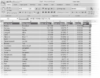
For example, using traditional formulas, to calculate the (approximate) age in years of each staff member, you would use a formula such as the one in cell G2 in Figure 21-22.

Figure 21-22: The formula in cell G2 uses an ordinary cell reference to D2.
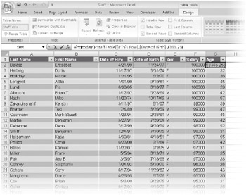
After you change the list to a table, you can edit the formula, and Excel will adjust the reference for you. Just select a cell with the formula, select the cell in the formula with the traditional single-cell reference, and then click the cell you are referring to (in this case, cell D2). Excel automatically replaces the cell address with the name of the table column, as you can see in Figure 21-23.

Figure 21-23: By turning the list into a table and editing the formula, we can turn the formula in G2 into something easier to read.
When you type the formula in the cell, Excel automatically copies the formula to the entire Age column, replacing all the existing formulas.
| Note | Excel will automatically replace all the formulas only if they are all equivalent. If you had created an exception formula somewhere in the list, Excel will put the formula into only the one cell, but it adds an AutoCorrect icon that asks whether you want to replace all the formulas in the column with the new formula. |
You might wonder about a few characteristics of the formula. First, why did Excel put brackets around the name of the column so it shows up as [Date of Birth]? Well, Excel needs something around the name, because otherwise the spaces in the name could make it hard to tell where the name ends. Simple parentheses wouldn't work well, because they are used in formulas to show calculation order. (Brackets are what Microsoft Office Access 2007 uses to identify column names, and it works pretty well in that application.)
Second, how does the formula know which row to use? In the original formula in cell G2, the reference was D2. When you copy the formula to cell G3, the reference changes to D3. The reference may be a little cryptic, but it's pretty clear the column and the row to which it refers. The reference [Date of Birth] tells which column, but how does Excel know which row? Notice in the traditional reference that the row number in the reference (for example, B2) was always the same as the row number of the cell that contained the formula (for example, G2). The people on the Excel team noticed that in many, many formulas-and especially in formulas in tables-the cell references point to other cells in the same row. So they created a rule. If the formula needs a single value (and the minus sign for subtraction needs a single value) and you give it a whole column as the reference, it will pick just the one from the current row. This is called implicit intersection because the formula implicitly uses the current row to intersect the range reference in the formula to get a single cell. (Excel will also implicitly intersect the current column with a horizontal range if necessary, but tables don't have horizontally named rows.)
Referencing the Total Row
Sometimes you need to refer to a row that's not the current row. For example, a common calculation in a table involves comparing the current row to the total row. For example, if your table includes sales by regions, you may want to show the percent each region is of the total. Or, because our Staff table example has the age calculated-with the average age in the total row-what if you want to know the age of each staff member compared to the overall average? Excel has a special way to represent the total row in a table formula.
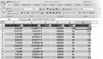
First, type a new heading so Excel will create a new column. Type something like Versus Avg. Then, after the new, formatted column appears in the table, select any cell in the column. Type an equal sign to start the formula, and click the Age column for the current row. The formula will say =[Age], showing that it recognizes the Age column. Then type a minus sign (-), and click the cell for the Age column in the total row. (As a keyboard shortcut, press the Left Arrow key to get to the Age column, and then press Ctrl+Down Arrow to jump to the bottom of the table-the total row.) The formula now says =[Age]-TStaff[[#Total],[#Age]]. When you press Enter, Excel inserts the formula into all the cells of the column. You can then apply a number format to the column. The result looks like the worksheet in Figure 21-24.

Figure 21-24: This formula uses structured referencing to compare the current row to the total row.
The syntax is a little bit scary, but once you get the hang of it, it's not too bad. The first part, =[Age], should be easy. That's just implicitly intersecting the Age column with the current row. The second part is a little trickier. In the reference TStaff[[#Total],[Age]], TStaff is just an arbitrary name assigned to the table. (See "Naming a Table" on page 671.) [#Total] is a special structured-reference tag that Excel automatically applies to the total row of the table. You can't use the [#Total] tag without first giving the name of the table (Excel wouldn't know which table you meant if you omitted this). So, the full reference has three parts: the name of the table (followed by square brackets), the special structured-reference tag [#Total], and then the column name [Age]. The [#Total] tag and the table column name are separated by a comma.
A structured reference is harder to write than it is to read. Fortunately, Excel will automatically create the structured-reference formula for you as you create new formulas that reference elements of a table.
Explicitly Referencing the Current Row
Implicit intersection lets you use column names in table formulas. It's a great feature and makes formulas much easier to understand and to write. The only time implicit intersection can be a problem is when you use a function that can accept a whole range but you want it to apply to only the current row. Implicit intersection kicks in only when the formula requires a single value-which is typical of arithmetic operations. But functions such as SUM can work just fine with a whole range. Suppose, for example, that you want to sum the scores for different parts of a test-but only for the current student. One way to do this is to simply select each cell separately and use the plus (+) sign to add them. In this way, implicit intersection will work.
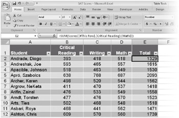
But if you have a lot of columns, using a range is easier. Fortunately, Excel has a special structured-reference tag, [#ThisRow], that explicitly limits the range to the current row. And Excel automatically adds that special tag when you create a formula that uses a function such as SUM over multiple columns of the current row. Figure 21-25 shows the formula Excel generates when you create a sum of multiple columns in the current row.

Figure 21-25: The [#This Row] tag tells Excel to total values from the current row only.
The formula =SUM(Scores[[#This Row],[Writing]:[Math]]) includes the standard SUM function. The reference follows the same pattern as when referring to the total row. There's the name of the table, followed by brackets. Within the brackets is the special structured-reference tag [#This Row], followed by a comma. Finally, there is the part that specifies the column. In this case, you're specifying a range of columns, so the formula uses the range (:) operator between two table column names.
Referencing Parts of a Table
In addition to the [#This Row] tag, whose explicit meaning changes depending on the cell containing the formula, Excel has four structured-reference tags for other parts of the table. Table 21-1 lists the tags, along with their meanings.
| Tag | Meaning |
|---|---|
| #Data | The data region of the table, excluding the header and total rows. If you refer to the table with no qualifier, this is what you get. |
| #Totals | The total row (if there is one). |
| #Headers | The header row (if there is one). |
| #AII | The entire table, including headers, data, and totals. |
These names are all row oriented. #Totals and #Headers reference single rows, but #Data and #A11 include all rows. If you combine any of these with a column name, you get the intersection. If you combine multiple row-oriented names, you get the union. For example, [#Headers],[#Data] results in everything except the totals.
Table 21-2 provides some example formulas that use the COUNTA function with structured-reference tags. Because each formula returns the total number of cells in a range, you can see how the different tags interact with one another. (All formulas reference a table named Staff.)
| Formula | Description |
|---|---|
| = COUNTA(Staff) | Number of data cells in the table body |
| = COUNTA(Staff[Salary]) | Number of data cells in the Staff column |
| = COUNTA(Staff[#Headers]) | Number of cells in the header row |
| = COUNTA(Staff[#Totals]) | Number of cells in the total row |
| = COUNTA(Staff[#Data]) | Number of data cells in the table (same as referencing the table name alone) |
| = COUNTA(Staff[[#Data],[Salary]]) | Same as referencing the column name alone |
| = COUNTA(Staff[#AII]) | Number of cells in the entire table, including the header and total row |
| = COUNTA(Staff[[#AII],[Salary]]) | Number of cells in one column, including header and total row |
| = COUNTA(Staff[[#Headers],[#Data]]) | Number of cells in the table, including headers but excluding the total row |
| = COUNTA(Staff[[#Headers],[#Data],[Salary]]) | Number of cells in one column, including headers but excluding the total row |
You can use the pointer to generate almost all of these combinations while constructing a formula. To select the #Data portion of the table, rest the pointer on the top-left corner of the table until it changes to a black arrow that points down and to the right, and then click once. To select the #A11 portion of the table, rest the pointer on the same place, but double-click. To select a column's #Data area, rest the pointer on the top of the column until it turns into a black arrow that points down, and then click once. To select the #A11 area for the column, rest the pointer on the same place, but double-click. To select the #Header and #Data combination, you have to manually edit the formula.
When you get used to the brackets, the structured references are much more meaningful than simple cell addresses. And if you change the size of a table, the structured names will automatically adjust. If you change the label in a column heading, any formulas that reference that column will automatically adjust.
| Note | How structured reference tags work is a lot more detailed, especially when you include special characters such as & or [ in the heading for a column. The details are described in the online Help topic "Using structured references with Excel tables." To find the topic, search for Structured References. |
EAN: 2147483647
Pages: 260