Filtering a List or Table

Filtering a list or table means hiding all the rows except those that meet specified criteria. Excel provides two filtering methods: Simple, which uses lists on the header row, and Advanced, which uses a separate criteria range. The Advanced method can filter in place or extract a subset to another part of the worksheet. You can use both methods with tables and also with standard lists-as long as the lists have header rows.

Using Filters

When you create a table, Excel adds filters to the header row automatically. To turn header row filters on or off, first select any cell in your table. Then click the Filter button in the Sort & Filter group on the Data tab. When you turn on the filter, Excel displays small arrows next to each of the column headings. Clicking the arrow next to any heading reveals a list of the column's unique values, which you can use to specify filtering criteria.

Inside Out-Display Arrows for Selected Columns

Sometimes, you want to apply filtering criteria to only one or two of your columns. If you're working with a standard list-not a table-you can select only the column headings you want to use as filters (the columns must be adjacent to one another). Then click the Filter button. This makes it clear which columns you are using for filtering.

Let's look at an example. Suppose that from the list shown in Figure 21-4 you'd like to see only those rows where the age is 33. To generate this subset, first make sure the filter arrows appear next to the column headings. If they don't, click the Filter button in the Sort & Filter group on the Data tab. Then click the small arrow next to the Age heading. Clear the Select All check box, then select the 33 check box, and finally click OK. The result looks like Figure 21-11.

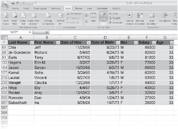
Figure 21-11: Use the filter lists to display only those rows in which the age is 33.

From the gaps in the row numbers shown in Figure 21-11, you can tell that Excel has hidden the rows that didn't meet the filtering criterion. To remind you that you have filtered your list, Excel also displays the filtered row numbers in a contrasting color.

As you can see from the selection list, you don't need to select a single item as a filter; you can select as many items from the list as you like. If you can see the item you want to sort by-for example, if you want to see all the rows with the age as 32, and you can see 32 in the list-just right-click the cell you want to match, click Filter, and then click Filter By Selected Cell's Value.

Determining How Many Rows Pass the Filter

Immediately after you add a new filter, Excel displays the number of rows that meet your criteria on the status bar. This information is ephemeral, however. Fortunately, you can use the SUBTOTAL function to arrive at this number. The easiest way to add the SUBTOTAL function is to turn the list into a table. If your list is not already a table, press Ctrl+T, and click OK. Even if you change it back to a range, you want it to be a table long enough to type SUBTOTAL formulas in a total row. After the list is a table, select the Total Row check box on the Design tab to create a total row with a default SUBTOTAL function. The default function displays a sum. To change it to a count, select any cell in the total row, and click the small arrow. Click Count. Otherwise, you can create the Subtotal function yourself.

For more information about the SUBTOTAL function, see "Adding Totals to a Table" on page 673.

Removing a Filter

To remove a filter from a single column, click the small arrow to the right of the column heading, and then click Clear Filter From Column. To remove all filters currently in effect, click the Clear button in the Sort & Filter group on the Data tab. To remove the filter arrows, click the Filter button in the Sort & Filter group on the Data tab. This removes the arrows from the header row cells. Converting a table to an ordinary range does automatically turn off the filters, but you can click the Filter button on the Data tab to turn the filters back on without turning the range back into an explicit table.

Using Filter Criteria in More Than One Column

You can specify filter criteria for your list in as many columns as you want. Filter your list on one column, filter the resulting list on another column, and so on. Each successive application of a filter refines the list further so that the result includes only those rows that meet all your criteria.

Note 

Basic filter operations always show only the rows that satisfy the criteria for all the filtered columns. If you want to see rows that pass either the filter for one column or the filter for another, you need to use the Advanced Filter command.

Using a Filter to Find the Top or Bottom n Items

You can use a filter to find the top or bottom n items in a numeric column or those items that make up the top or bottom n percent of a column's total. Click the arrow for the column, click Number Filters, and then click Top 10. The dialog box shown in Figure 21-12 appears.

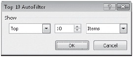
Figure 21-12: Use the Top 10 Filter dialog box to zero in on the top or bottom n list elements.

The Top 10 Filter dialog box has three boxes. In the first, you can select either Top or Bottom. In the second, you can specify any number from 1 to 500. In the third, you can select either Items or Percent.

Using a Filter to Display Blank Entries

If a column contains blank cells, you find a Blanks check box at the bottom of its filter list. (You open this list by clicking the small arrow to the right of the column header.) If you want to locate those rows in which a particular column has no entry, select the Blanks check box as your criterion.

Using Filters to Select Dates

Dates can often be frustrating to filter because you usually want to filter based on some kind of grouping. You don't just want March 13, 2008. You want all of March. So in the past, it was usually necessary to create additional columns in the list to calculate just the month or just the year so that you could use those columns as filters. Also, when filtering by dates, you often want to filter by dates that are relative to now. For example, you want to see the orders from last month, the plan for next year, or the invoices so far this year. Excel 2007 includes filter capabilities to make all these tasks really simple.

If the column you are filtering by contains dates, the selection list automatically groups the dates into months and years. Click the small arrow for a column that contains dates, and you now see a list of years. You can then expand the years to see months:

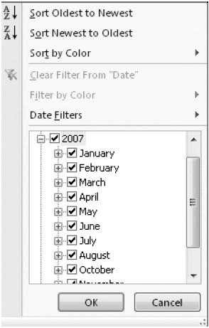
To see individual dates for a month, expand the month heading.

In addition, clicking the Date Filters command in the Filter list gives you many date-specific options, including many that compare the date to the current day-such as Next Month or Last Month.

Using Filters to Specify More Complex Criteria

The example in Figure 21-11 used a single equality comparison for its criterion. That is, we asked Excel to display only those rows in which the Age field was equal to a particular value, 33. Each data type column now has a specialized list of the functions most common to that data type:

• Number filters include comparisons such as Greater Than, Between, and even Above Average.

• Date filters include comparisons such as Yesterday, Next Year, and All Dates In Quarter 1 (regardless of year).

• Text filters include comparisons such as Begins With and Contains.

These data type-specific filtering options can handle most of your basic needs.

Using Custom Filters to Specify Complex Relationships

If you want to get even more complex, you can use the Custom Filter command. To access this command, click the small arrow to the right of a column heading, click the data type-specific menu (such as Number Filter or Data Filter), and then click Custom Filter. The Custom Filter dialog box shown in Figure 21-13 appears. For numeric and date fields, the Custom Filter command is most useful when you use the keyword or with two nonequal comparisons in the same column-for example, all the age values less than 25 or greater than 65. For text columns, the Custom Filter command lets you create between ranges and lets you use sophisticated wildcard comparisons. For example, you might create a filter to find names with A as the first letter and e as the third letter.

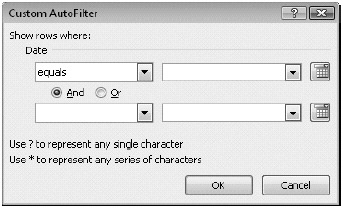
Figure 21-13: Use the Custom Filter dialog box to apply more complex filter criteria to a single column.

You can enter one or two criteria in the Custom Filter dialog box, and you can select from a full range of Excel relational operators. The list boxes on the left side of the dialog box provide a selection of relationships (Equals, Does Not Equal, Is Greater Than, and so on), and the list boxes on the right let you select the values that appear in your list. You can, of course, type directly in the boxes on the right, if you prefer that to fishing through the list for a value.

Suppose, for example, that you want to see all the members of your Staff list with salaries greater than or equal to 90,000 as well as all those with salaries less than or equal to 30,000. After displaying the Custom Filter dialog box for the Salary column, select Is Greater Than Or Equal To in the upper-left box, and type 90000 in the upper-right box. Select the Or option, select Is Less Than Or Equal To in the lower-left box, and type 30000 in the lower-right box. If you neglect to select the Or option, you ask Excel for the names of employees who made both 90,000 or more and 30,000 or less, and you get an empty list.

Finding an Alphabetical Range of Text Values To find all the text values in a column that fall within a particular range of letters, use the Custom Filter dialog box, and specify two criteria joined by And. For example, to find all last names beginning with B, C, or D, filter the Last Name column, and specify Is Greater Than B and Is Less Than E in the Custom Filter dialog box.

Using Wildcards in Custom Criteria The Custom Filter dialog box accepts two kinds of wildcard characters. You can use the asterisk (*) to represent any sequence of characters or the question mark (?) to represent any single character. For example, to find all last names starting with B, you can specify Is Equal To B* in the Custom Filter dialog box. To include a literal question mark or asterisk in a filter, precede the ? or * with a tilde (~).

Using the Advanced Filter Command

In contrast to the Filter command, the Advanced Filter command lets you do the following:

• Specify criteria involving two or more columns and the conjunction OR.

• Specify three or more criteria for a particular column, where at least one OR conjunction is involved.

• Specify computed criteria (for example, all employees whose salaries are more than 25 percent greater than the median salary).

• See in printable form the filters that are applied to the list or table.

In addition, you can use the Advanced Filter command to extract rows from the range, placing copies of those rows in another part of the current worksheet. As with a regular filter, you can use Advanced Filter whether you turn the list into a table or not. Some features-such as showing totals at the bottom-are much easier if you turn the list into a table.

TROUBLESHOOTING 

I can't extract to a separate worksheet.

You cannot extract rows from a list and place them on a separate worksheet. Your criteria range can be on a different worksheet, but your extract range cannot. After you extract a set of rows, you can, of course, copy or move it to another location.

Specifying a Criteria Range

The Advanced Filter command, unlike the standard filter, requires that you specify filtering criteria in a worksheet range separate from your list or table. Because entire rows are hidden when the filter is executed, it's inadvisable to put the criteria range alongside the list. Instead, put it above the list or on a separate worksheet. A criteria range must consist of at least two rows. Type one or more column headings in the top row, and type your filtering criteria in the second and subsequent rows. With the exception of computed criteria, you must spell the headings in your criteria range exactly like those in your list. (Capitalization and formatting don't have to match, but spelling does.) To ensure accuracy, the best way to create these headings is by selecting the column headings in your list and then using the Copy and Paste commands.

Keep in mind that a criteria range does not have to include headings for every column in the list. Columns that are not involved in the selection process don't have to be part of the criteria range.

An Example Using Two Columns Joined by OR

Figure 21-14 shows a list of homes for sale. (The underscored items in column A are hyperlinks to pictures of the houses.) Suppose you're interested in homes with lot size (column H) of at least 2 acres. You'll also consider homes on smaller lots if they're in the elementary-school district U (column O). To filter the list so that homes meeting either criterion are shown, begin by creating the criteria range shown in Figure 21-15. We've created this criteria range above the list, on three newly inserted rows.

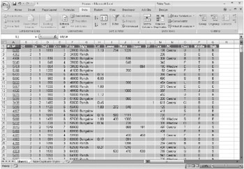
Figure 21-14: Use the Advanced Filter command to locate homes within this list that meet specific criteria.

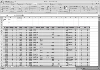
Figure 21-15: This criteria range filters the list to show homes that are either on lots of at least 2 acres or within elementary-school district U.

On the CD You'll find the  Homes.xlsx file in the Sample Files section of the companion CD.

You then click Advanced Filter in the Sort & Filter group on the Data tab and fill out the Advanced Filter dialog box, as shown in Figure 21-16. Excel responds by displaying the filtered list shown in Figure 21-17. Some of the Lot fields in that filtered list are blank because the original list didn't include lot-size information about all the homes. Excel treats the blanks as zeros (and therefore less than 2) and includes them only if their Elem fields contain U.

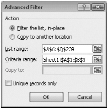
Figure 21-16: In the Advanced Filter dialog box, select Filter The List, In-Place, and specify the addresses of your list and your criteria ranges.

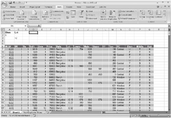
Figure 21-17: Excel responds with a list filtered to show just the homes in which you're interested.

Like a standard filter, the Advanced Filter command hides all rows that don't pass the filter. It also displays the qualifying row numbers in a contrasting color. As with a regular filter, it's worth making the list into a table if you want to add a total row. On the total row, you can easily add a COUNT function to see how many rows passed the filter.

In Figure 21-15, notice that we specified the two criteria on separate lines. This tells Excel to find rows that meet either criterion. If you put the two criteria on the same line, you ask for just those rows that meet both criteria. In other words, criteria on the same line are joined by AND, and criteria on separate lines are joined by OR. You can put as many separate criteria as you like in a criteria range.

We specified both criteria as simple text values. The value U under the Elem heading tells Excel to get any rows with Elem values that begin with the letter U. (In other words, there's an implied asterisk wildcard after the U.) If you want the filter to allow only values that match the letter U exactly, you type ="=U". This clumsy-looking formulation causes the cell to display =U and has the effect of removing the implied asterisk wildcard.

The value >=2 under the Lot heading tells Excel to get rows with Lot values equal to or greater than 2. You can use any of the relational operators >, <, >=, or <= in a numeric criterion. If you want an exact match (all lot sizes of exactly 2 acres, for example), type the number without an operator.

Be aware that a blank cell in a criteria range means "accept any value for this column." If you accidentally include a blank row in the criteria range, you get an unfiltered list.

Note 

Provided your criteria range is on the same worksheet as your list, Excel assigns the name Criteria to it immediately after you use it. You can use this behavior as a navigational tool. If you need to return to a criteria range to edit it, you can get there by pressing F5 and selecting Criteria in the Go To dialog box.

An Example Using Three ORs on a Column

Now let's suppose you want to filter the list to show all houses in three elementary-school districts-U, F, and T. You include only the Elem field in the criteria range and type the letters U, F, and T on three separate rows immediately below the heading. The Advanced Filter command then generates the list shown in Figure 21-18.

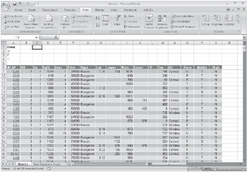
Figure 21-18: Using the criteria range in cells A1-A4 reduces the list to those houses in elementary-school districts U, F, and T.

An Example Using Both OR and AND

If you want to see all houses in middle-school district T or J that are at least 2,000 square feet, you set up the criteria range as in Figure 21-19. The criterion >=2000 appears in cells B2 and B3, because for each of the middle-school districts (T and J), you want to see houses only of 2,000 square feet or more.

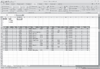
Figure 21-19: To display 2,000-square-foot houses in middle-school districts T and J, repeat the >=2000 criterion in each line of the criteria range.

Note 

Each time you use the Advanced Filter command, Excel reexamines the entire list rather than only the rows that passed the most recent filter. Therefore, you don't have to use the Clear command before changing the filter. If you want to refine a filter set-that is, filter the filtrate-add your new criteria to the previous criteria range and filter again.

Applying Multiple Criteria to the Same Column

To apply two or more criteria to the same column, repeat the column in your criteria range. For example, to retrieve rows with Price values from 50,000 to 90,000, your criteria range would look like this:

Price	Price
>=50000	<=90000

To exclude rows with prices in this range but admit everything else, you'd set up this criteria range:

Price	Price
<=50000	>=90000

Using Computed Criteria

Computed criteria involve any test other than a simple comparison of a column's value to a constant. Asking Excel to find houses with prices less than $200,000 does not require a computed criterion. Asking for houses with prices less than the median price of all houses in the list does.

When setting up a computed criterion, observe these rules:

• The column heading above a computed criterion must not be a copy of a column heading in the list. This heading can be blank, or it can be anything you want-other than a heading that already appears in the list.

• References to cells outside the list should be absolute.

• References to cells inside the list should be relative-unless you're referencing all the cells in a column.

Let's look at some examples. The next three sections explore referencing cells within the list, referencing a cell outside the list, and referencing all rows in a column.

Referencing Cells Within the List In cell A2 of Figure 21-20, we used the formula =F6/D6<50 to find all houses with prices per square foot less than $50. Notice that the heading above the criterion (at cell A1) is not a copy of any heading in the list and that the formula uses relative references to fetch values from within the list. F6 and D6 are the relevant values from the first row of the unfiltered list. Excel therefore begins by dividing F6 by D6 and comparing the result to 50. Because the references are relative, it continues by dividing F7 by D7, dividing F8 by D8, and so on.

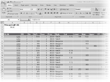
Figure 21-20: The criterion in A2 returns all houses with prices per square foot less than $50.

The formula in A2 happens to return TRUE, because the result of that initial calculation (involving F6 and D6) is TRUE. It doesn't make any difference what that criterion formula returns, however; in fact, as you'll see, it can even return an error value.

In some rows of the unfiltered list, the SqFt column is blank. Dividing by a blank cell always returns the #DIV/0! error constant. This is not a problem. When Excel looks at a row with a blank SqFt value, it compares #DIV/0! with 50, and the result of that comparison is #DIV/0! Because the comparison doesn't yield a TRUE result, the row containing the blank SqFt value is excluded from the filter set-which is, presumably, the outcome you want.

If you've assigned names to the columns of your list, you can use those names instead of first-row cell references in your computed criterion. In other words, with the names SqFt and Price assigned to the appropriate columns, the formula at A2 reads =Price/SqFt<50.

Referencing a Cell Outside the List The criterion formula in A2 of Figure 21-21 compares prices against the median price, which is stored outside the list, in H1. (The median is calculated with the formula =MEDIAN(price), where price is a name assigned to all cells in the Price column.) The reference to H1 is absolute. If it were not, Excel would compare the price in the first row of the list to H1, the price in the second row to H2, and so on-not what you want.

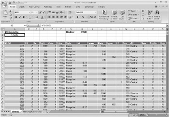
Figure 21-21: This criterion in A2 uses an absolute reference, because the referenced cell, H1, lies outside the list.

Referencing All Rows in a Column If you change the formula in A2 of Figure 21-21 to =F6>MEDIAN($F$6:$F$238), you get the same set of rows as shown in Figure 21-21. In this case, the MEDIAN function references cells within the list, but the reference has to be absolute. Otherwise, Excel looks at F6:F238 and then at F7:F239, and so on. (You could drop the absolute reference to column F and make the row references absolute. If you use the F4 shortcut to create the absolute references, however, it's just as easy to make the whole reference absolute.)

Extracting Filtered Rows

The Advanced Filter dialog box includes an option for copying the selected rows to another worksheet location, instead of displaying a filtered list. To copy rows rather than display them, select the Copy To Another Location option in the Advanced Filter dialog box, and supply the name or address of the range where you want the information to appear in the Copy To text box.

The easiest way to specify the Copy To range is to click a blank cell in your worksheet where you want the range to start. Be sure the cell has plenty of blank space below and to the right of it. Excel then copies your list's column headings and all the rows that meet the Advanced Filter criteria to the range that begins with the cell you specified. Be careful, though; any data already stored in the selected range will be overwritten. Alternatively, if you specify a range of cells, Excel copies the rows that pass the filter but stops when the range is full.

If you put the extract range to the side of the source list, be careful not to filter the source list. Filtering the source list hides the entire rows, which will hide rows from your extract range as well. Be sure to either turn off any in-place filters in the source list or put the extract range below the source range. Now that Excel 2007 allows a million rows, you should have plenty of room below most lists. The extract range has to be on the same worksheet as the source list, but after you have extracted the list, you can move it to a different worksheet.

Note 

When you specify a Copy To range in the Advanced Filter dialog box, Excel assigns the name Extract to that range. You can use this name as a navigational aid. For example, when you need to return to the range to change column headings, select Extract from the Name box to the left of the formula bar.

To copy only certain columns of your list to a new location, create copies of the headings for those columns. Then specify the headings (not only the first cell but the entire set of copied headings) as your Copy To range. Be sure not to select a blank row under the extract headings, or you will get only a single row from the filter.

The Unique Records Only Check Box The Unique Records Only check box in the Advanced Filter dialog box adds a filter to whatever you specify in your criteria range. It eliminates rows that are duplicates in every respect (not just duplicates in the columns that you happen to be extracting, but duplicates in all columns). The Unique Records Only check box works only in conjunction with the Copy To Another Location option; this option is particularly useful when you are extracting only some of the columns. For example, you could extract only the Price and Style columns. By using the Unique Records Only check box, you would get a list of unique Price/Style combinations from the list.

Removing Duplicate Records

In previous versions of Excel, one reason for using the Unique Records Only check box was to eliminate duplicates from a list. Now that task is much easier, because a special command simply removes duplicate rows from the list. You can use this command in two ways. One way is to simply remove all the duplicate rows-in case there happen to be any. The other way is to select specific columns that you will force to be unique. When you select specific columns, Excel simply chooses the values from all the other columns that happen to be in the first unique combination.

To remove complete row duplicates, select a single cell within the list or table, and click the Remove Duplicates command in the Data Tools group on the Data tab. In the Remove Duplicates dialog box, leave all the check boxes for the columns selected, and click OK. Excel will tell you how many duplicates it found and how many rows are left.

To remove partial-row duplicates, you will probably want to start by making a copy of the list, because real information will be destroyed in the process. Next, you should sort the list for any columns that you will not include. For example, if you want only one row for each home style but you want that row to be the most expensive home, sort the list in descending order by Price before you execute the Remove Duplicates command.

After you have sorted the list, select a single cell, and click Remove Duplicates. Click the Unselect All button to clear all the check boxes, and then select the check boxes for the few columns in which you want distinct values. For example, you might select only the Style column. Then click OK. You'll end up with a list that contains only the first row for each style-the most expensive, if you sorted the list first.