Creating a Table

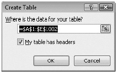
After you have some data in a worksheet range, you can designate that range as a table by selecting any cell within it and pressing Ctrl+T or Ctrl+L. That's the easy way. If you want to work a little harder, you can click Table in the Tables group on the Insert tab. Either way, start by selecting a single cell anywhere in the table range before issuing the command. Excel will figure out the dimensions of the table for you and ask for confirmation in the Create Table dialog box:

Unless the program has made some kind of mistake, you can click OK to create your table. If you select more than one cell but less than the entire range before pressing Ctrl+T, Excel will try to create a table out of the specific cells you selected.

Note 

Many new features of Excel tables do not work if your workbook is opened in Compatibility mode. You must convert a workbook you have saved with the type Excel 97-2003 Workbook to an Excel 2007 workbook in order to get the new functionality. See "File Formats" on page 54 for details about converting an existing workbook into native Excel 2007 format.

Overwriting Default Headers

Notice that, in addition to recognizing the size of the table, Excel figures out whether the top row of your range is a header row-a row of column labels. If your range does not include such a row or if for some reason you choose to clear the My Table Has Headers check box in the Create Table dialog box, Excel will create a header row for you using labels such as Column 1, Column 2, and so on. Default headers like these are both ugly and pointless; it's far better to set up your own descriptive headers before creating the table. But if you omit this step, you can always override the defaults later by selecting the header cells and typing over them, just as if they were ordinary worksheet cells. (They're not quite ordinary data, actually; Excel won't let you delete them, and if you try to clear a header, you'll just get the default back.)

Turning a Table Back into an Ordinary Range

If the need arises to turn a table back into an ordinary worksheet range, select any cell or block of cells within the table. Then click Convert To Range in the Tools group on the Design tab. Click Yes to answer the confirmation prompt. Note that after you change a table into a regular range, the formatting turns into regular cell formatting. This can cause unexpected behavior if you ever turn the range back into a table. See the "Formatting Tables section on page 705 for details about managing table and cell formatting.

Inside Out-Check the Ribbon

An easy way to tell whether a range is a table is to select a cell in the range and look at the Ribbon. If you see a Table Tools tab, then the current list has been converted to a table.

Naming a Table

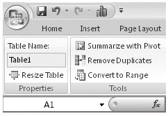
When you designate a range as a table, Excel assigns a name to that table and displays the name in the Properties group on the Design tab:

As this example shows, Excel uses default names (Tablel, Table2, and so on) unless you supply your own names. Does the name matter? Perhaps. Formulas that take advantage of structured referencing use the table name, and a descriptive name serves the purpose of self-documentation better than a default name. In the following formula, for example:

 =SUM(Scores[Math]) 

the word Scores is the table's name. (The formula sums the values from the Math column of the Scores table.)

Giving a meaningful name to the table is particularly useful when you have multiple tables on a single worksheet and have formulas that refer to the tables. By using names for the tables, you can instantly tell when looking at a formula which table it is referencing.

It's definitely worthwhile to assign an intelligible name to your table if you think you might at some point record or write a macro that references the table. That way your macro code will be easier to understand (easier for you and easier for anyone else who sees your code). Moreover, if you record a macro that references Table1 and you subsequently name the table SurveyData, your macro will no longer perform as expected and will cause you considerable vexation. It's best to form the habit of naming objects when you create them.

To change a table's current name (default or otherwise), select a cell within the table, and click the Design tab. Then type in the Table Name box in the Properties group.

Expanding a Table

To add a new row to the end of a table, go to the bottom-right cell of the table (ignoring the total row, if there is one), and press Tab. Excel will extend the table for you, no questions asked, copying all formatting and formulas in the process. When you get to the last column in the new row, press Tab to create yet another new row. Thus, after you have created the stub of a table, you can expand it downward by simply typing in the usual way and pressing Tab between cells (or at any rate at the end of each row).

Note that pressing Tab creates a new table row above the total row, if your table has a total row. The total row simply moves down one row to accommodate your new data, and Excel updates the formulas appropriately. (For more about the total row, see "Adding Totals to a Table" on the next page.) If you don't have a total row in your table, you can also extend the table by simply typing in the blank row below the bottom row of the table. Using Tab to extend the table works whether you have a total row or not.

Automatic expansion works for columns as well as rows. If you type in any row of the column directly to the right of a table, Excel expands the table to include the new column. If the new data is a formula, the formula is replicated throughout the column.

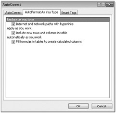
If you don't want the table to automatically expand or automatically fill columns with formulas, you can turn off the option. Click the Microsoft Office Button, and then click Excel Options. Select the Proofing category, and click AutoCorrect Options. In the Auto-Correct dialog box, shown in Figure 21-2, click the AutoFormat As You Type tab. Clear the Include New Rows And Columns In Table check box to prevent Excel from expanding the table, and clear the Fill Formulas In Tables To Create Calculated Columns check box to prevent Excel from filling entire columns with identical formulas.

Figure 21-2: Use the AutoCorrect dialog box to control table expansion.

If you're not currently displaying a total row with your table, you'll find a minuscule handle in the lower-right corner of the cell occupying the lower-right corner of your table. This handle gives you yet another way to expand your table. Usually, it's easier just to add data and let Excel expand the table. But if you want to add several new rows or columns all at once, the handle is a good way to do it.

Selecting Rows and Columns Within a Table

Excel makes it easy to select rows and columns within a table. If you rest the pointer on the left edge of the first cell in a row, the pointer changes to a solid arrow. Click once, and you've selected the row. If your table happens to begin in column A of the worksheet, be sure you rest the pointer inside the first cell, rather than on the worksheet frame. On the frame, the pointer also changes to a solid arrow, but clicking here will select the entire worksheet row.

To select a column, rest the pointer near the top of the column's heading, and then click. Clicking once selects the column's data, excluding the header and the total (if you have displayed the total row). Clicking a second time selects the entire column-header, data, and total.

To select the entire table, rest the pointer on the upper-left corner of the first column's header. When you see the pointer turn southeast, click. Click once for the data only or twice for everything-data, headers, and totals.

Selecting with the keyboard is even easier, particularly with a large table when the top and left edges are out of sight. Pressing Shift+Spacebar selects the current row, regardless of which cell is selected. Pressing Ctrl+Spacebar selects the current column's data, omitting the header and total. Pressing Shift+Ctrl+Spacebar or Ctrl+A selects all the table's data.

Multiple key presses expand the selection predictably: Pressing Shift+Spacebar twice selects the entire current worksheet row. Pressing Ctrl+Spacebar twice selects the current table column, with the header and total. Pressing Ctrl+Spacebar three times selects the entire current worksheet column. Pressing Shift+Ctrl+Spacebar or Ctrl+A twice gets the entire table, headers, and totals included. Pressing that combination a third time selects all gazillion cells of the worksheet.