Normalizing Vectors

What Is a Parametric Equation?

In Chapter 1, I started with a line as the simplest example of a polynomial curve and I gave the equation for a line in terms of its slope and an offset. This is a mathematically correct form, and the form you usually learn first in school, but it is also fairly limited in how it can be used in practical applications because it doesn't explicitly handle some of the issues that come up when you are writing code.

For example, a math teacher will tell you that a vertical line has a slope that is undefined because of the "rise over run" definition of the slope. This is mathematically true, but it is inconvenient to think of your rocket ship as traveling along a path that is "undefined". Also, the simple equation for a line is not explicitly bounded by two endpoints, yet nearly all lines you draw will be based on explicit endpoints. For these and other reasons, it would be advantageous to have an alternate representation for a line.

This is where parametric equations come in handy. Imagine the following scenario. I tell you to walk from point A to point B beginning at time t=0 and ending at time t=1. Your position, P, at any given time throughout your journey will be a function of A, B, and t, as shown in Figure 3.1.

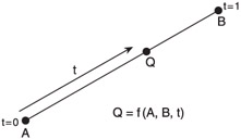
Figure 3.1: Describing a path along a line.

If you wanted to use the line equation from Chapter 1, you could use the two points to find the slope and the offset. You could then have an equation that defined y in terms of x. If you wanted to find point Q, you'd have to choose a value for the x component of point Q and then compute the y component. If the slope is undefined, you would have to account for that as a special case. Instead, Figure 3.1 shows that you can formulate a line equation based on a parameter, t. The result is a parametric form of the line equation as shown next .

(3.1) The parametric equation for a line. 

My example implies that the variable t stands for time. In some cases this might be true, but it is more generally true to think of t as the normalized distance along the length of the path formed by the two endpoints. So, you can find the location of any point along the line with Equation 3.1. This can be convenient because you can think in terms of the line itself. For instance, the position of the midpoint becomes trivial. Simply use 0.5 for the value of t.

It should also be clear that the parametric form obviates the need to handle vertical lines with special code. Equation 3.1 works equally well for lines of any orientation. Also, it works well for lines in any number of dimensions. Equation 3.1 does not explicitly refer to x and y values because the same form is useful for 2D lines, 3D lines, or even higher. However, just to be clear, Equation 3.2 shows a more detailed view of how you compute the actual points.

(3.2) Computing the output of the parametric equation.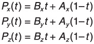 

So, the parametric form allows you to think of curves as functions of a set of control points and a parameter that corresponds to a distance along the length of the curve. As you will see in this chapter and most of the others, this form is much more flexible and powerful than the form you learned in Chapter 1 or your math classes. Having said that, the concepts in Chapter 1 are still valuable because parametric functions are still polynomials . The only difference is that they are now polynomial functions of t instead of x. All the rules in Chapter 1 and Appendix A hold true for parametric equations. In fact, before I move on to actual curves, I should talk a little bit about how to find the derivative of a parametric equation.