Extending the Data Analysis Features in Microsoft Excel

Because many of the Excel data analysis tasks that you will do on a daily basis involve sorting, filtering, and subtotaling data records, let’s start with an example of how to automate these straightforward tasks. The code we’ll examine in the next several sections is attached to the BookSale.xls file in the Chap11 folder. If you want to run the code samples as you read, go ahead and open the file now.

Sort, Filter, and Subtotal Lists of Records

You can use code similar to the following SortSales subroutine to sort a list of data records. Using code such as this is a good way to ensure that records are always sorted when an Excel workbook is opened.

Public Sub SortSales() ’ Purpose: Sorts a list of book store sales in descending order. Dim objWorksheet As Excel.Worksheet Dim objRange As Excel.Range ’ Select the list. Set objWorksheet = Excel.Application.ActiveWorkbook.Sheets _ (Index:="Book Store Sales”) Set objRange = objWorksheet.Range(Cell1:="A1", Cell2:="D37”) ’ Sort the list. objRange.Sort Key1:=objWorksheet.Range(Cell1:="D1”), _ Order1:=xlDescending, Header:=xlYes Set objRange = Nothing Set objWorksheet = Nothing End Sub

Here’s how the SortSales subroutine works:

• As you’ve already learned, the keyword Public means that the subroutine is available to any other procedures in the code project. The Sub keyword indicates that the procedure does not return any value to any calling procedure.

• Here again, the Dim keyword reserves a memory location, using the name that follows each statement. Each memory location is dimensioned large enough to hold an object of the type following the As keyword. In this case, the memory locations are large enough to hold a Worksheet object and a Range object.

• The Set keyword is used to put something inside the corresponding memory location. In this case, the code

  Set objWorksheet = Excel.Application.ActiveWorkbook.Sheets _ (Index:="Book Store Sales")

means that the memory location objWorksheet, representing a Worksheet object, will hold a reference to the worksheet named Book Store Sales in the active Excel workbook. At the end of the subroutine, the memory locations’ contents are emptied and released to other computer processes by setting the object variables, such as objWorksheet, to Nothing.

Note

The Public, Sub, Dim, As, Set, and Nothing keywords are used in the same manner as described here and earlier in the remaining code samples, so I’ll no longer describe them in detail.

• In Excel, a Range object can be used to refer to a group of cells on a worksheet; in this case, the cell range A1 to D37, inclusive. To refer to a single cell, use the Worksheet object’s Range method with only the Cell1 argument specified.

• The Range object’s Sort method can be used to sort the group of cells referred to in the Range object. In this code, the Sort method’s Key1 argument specifies that the column header in cell D1 (Sales) is the basis of the sort. The Order1 argument specifies a descending sort order by using the xlDescending constant. The Header argument is set to xlYes to ensure that cell D1 is not sorted along with the rest of the column’s cells.

You can run the SortSales subroutine by clicking anywhere inside the subroutine’s code and clicking Run Sub/UserForm on the Run menu. You can also call the procedure from the ThisWorkbook module’s Workbook object’s Open event by adding the following code to the ThisWorkbook module:

Private Sub Workbook_Open() Call SortSales End Sub

To run the SortSales subroutine using this method, close the workbook and then reopen it. When the workbook is opened, the SortSales subroutine automatically runs. Figure 11-5 shows the result of running the SortSales subroutine.

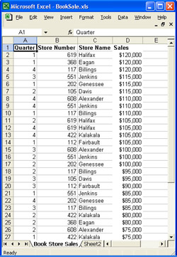
Figure 11-5: Results of running the SortSales subroutine.

You can use code similar to the following subroutine, named FilterSales, to filter a list of data records. Like the SortSales subroutine, this subroutine is a good way to ensure that records appear as you need them when an Excel workbook is opened.

Public Sub FilterSales() ’ Purpose: Filters a list of book store sales by displaying ’ only sales above $100,000. Dim objWorksheet As Excel.Worksheet Dim objRange As Excel.Range ’ Select the list. Set objWorksheet = Excel.Application.ActiveWorkbook.Sheets _ (Index:="Book Store Sales") Set objRange = objWorksheet.Range(Cell1:="A1", Cell2:="D37") ’ Filter the list. ’ 4 is the Sales column. objRange.AutoFilter Field:=4, Criteria1:=">100000" Set objRange = Nothing Set objWorksheet = Nothing End Sub 

The FilterSales code is almost identical to the SortSales code. The exception is the line of code objRange.AutoFilter Field:=4, Criteria1:=“>100000”. In this case, the Range object’s AutoFilter method is using the Field argument to specify the column number to filter on (the 4th column, column D). The Criteria1 argument specifies that only records with values of greater than 100,000 in column D should be displayed. The result of running the FilterSales subroutine is shown in Figure 11-6.

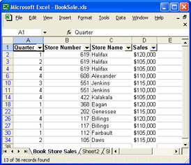
Figure 11-6: Records filtered by running the FilterSales subroutine.

In like manner, the CreateSubtotals subroutine, shown in the following code, can be used to automatically subtotal a list of records.

Public Sub CreateSubtotals() ’ Purpose: Creates subtotals for a list of book store sales records. Dim objWorksheet As Excel.Worksheet Dim objRange As Excel.Range ’ Select the list. Set objWorksheet = Excel.Application.ActiveWorkbook.Sheets _ (Index:="Book Store Sales") Set objRange = objWorksheet.Range(Cell1:="A1", Cell2:="D37") ’ Subtotal the list. ’ 2 is the Store Number column, and 4 is the Sales column. objRange.Subtotal GroupBy:=2, Function:=xlSum, TotalList:=4 ’ Collapse the outline to show only the subtotals. objWorksheet.Outline.ShowLevels RowLevels:=2 Set objRange = Nothing Set objWorksheet = Nothing End Sub 

Two lines of code differentiate the CreateSubtotals subroutine from the SortSales and FilterSales subroutines.

• The line objRange.Subtotal GroupBy:=2, Function:=xlSum, TotalList:=4 uses the Range object’s Subtotal method to display the subtotals. The GroupBy argument specifies the second column (the Store Number column) as the record grouping for subtotals. The Function argument uses the xlSum constant to specify that the subtotals are sums. The TotalList argument specifies the fourth column (the Sales column) as the basis of the sums.

• The line objWorksheet.Outline.ShowLevels RowLevels:=2 is used to collapse the displayed subtotal level. The code uses the Worksheet object’s Outline object, which contains a ShowLevels method; the method’s RowLevels argument is set to 2, which specifies that the second subtotal level is to be displayed. Setting this argument to 2 is equivalent to clicking the 2 icon in the subtotals navigation column.

The result of running the CreateSubtotals subroutine is shown in Figure 11-7.

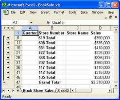
Figure 11-7: Subtotals added by running the CreateSubtotals subroutine.

Insert Standard Excel Worksheet Functions and Analysis ToolPak Functions

Worksheet and Analysis ToolPak functions bring a greater degree of analysis to your data than sorting, filtering, and subtotaling. For example, you might want to use code to insert and run a worksheet function or Analysis ToolPak function whenever a particular series of numbers changes or exceeds a certain threshold. The following subroutine (named InsertWorksheetFunctions) demonstrates how to insert a SUM and AVERAGE function into the Book Store Sales worksheet in the BookSale.xls file in the Chap11 folder.

Public Sub InsertWorksheetFunctions() ’ Purpose: Inserts worksheet functions into the book store sales list. Dim objWorksheet As Excel.Worksheet Dim objRange As Excel.Range Dim objFunctionResult As Excel.Range Dim objLabel As Excel.Range ’ Select the numbers to calculate. Set objWorksheet = Excel.Application.ActiveWorkbook.Sheets _ (Index:="Book Store Sales") Set objRange = objWorksheet.Range(Cell1:="D2", Cell2:="D37") ’ Indicate where to insert the function’s result. Set objFunctionResult = objWorksheet.Range(Cell1:="D38") ’ Sum all of the sales in column D. objFunctionResult.Value =_ Excel.Application.WorksheetFunction.Sum(objRange) ’ Insert a descriptive label. Set objLabel = objFunctionResult.Offset(ColumnOffset:=-1) objLabel.Value = "Sum of Sales" ’ Average the sales in column D. Set objFunctionResult = objWorksheet.Range(Cell1:="D39") objFunctionResult.Value = _ Excel.Application.WorksheetFunction.Average(objRange) ’ Insert another descriptive label. Set objLabel = objFunctionResult.Offset(ColumnOffset:=-1) objLabel.Value = "Average of Sales" Set objLabel = Nothing Set objFunctionResult = Nothing Set objRange = Nothing Set objWorksheet = Nothing End Sub 

Although the InsertWorksheetFunctions subroutine has quite a few lines of code, the operations it performs are straightforward.

• The lines of code starting with Set objFunctionResult specify the cells in which the results of each function will appear. The SUM function result will appear in cell D38, and the AVERAGE function result will appear in cell D39; the result is specified by the Range object’s Value property. In this case, the WorksheetFunction object’s Sum method calculates the sum of cells D2 through D37 (the Sales column) and places the result in cell D38. The WorksheetFunction object’s Average method calculates the average of cells D2 through D37 and places the result in cell D39.

  Note

  The WorksheetFunction object contains over 175 methods representing a wide array of Excel worksheet functions.

• The lines of code starting with Set objLabel and objLabel.Value specify that a descriptive label for each function result be placed one cell to the left of the function result. The code performs this operation by setting the ColumnOffset argument of the Range object’s Offset property to -1 (a value of 1 would offset one column to the right).

The result of running the InsertWorksheetFunctions subroutine is shown in Figure 11-8.

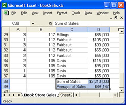
Figure 11-8: Results of running the InsertWorksheetFunctions subroutine.

For more sophisticated worksheet calculations, you can use the Analysis ToolPak functions. To do so, you must first set a reference to the Analysis ToolPak VBA functions. The steps to add the reference are described in the code comments below. The InsertAnalysisToolPakFunctions subroutine automatically runs the Descriptive Statistics and Rank and Percentile tools against data records in the BookSale.xls file.

Public Sub InsertAnalysisToolPakFunctions() ’ Purpose: Inserts Analysis ToolPak functions into ’ the book sales worksheet. ’ Note: You must first reference the Analysis ToolPak VBA functions. ’ To do so: ’ In Excel, on the Tools menu, click Add-Ins. ’ Select the Analysis ToolPak–VBA check box. ’ In the Visual Basic Editor, on the Tools menu, click ’ References. Select the atpvbaen.xls check box, and then click OK. Dim objWorksheet As Excel.Worksheet Dim objRange As Excel.Range Dim objOutput As Excel.Range ’ Select the list and output location. Set objWorksheet = Excel.Application.ActiveWorkbook.Sheets _ (Index:="Book Store Sales") Set objRange = objWorksheet.Range(Cell1:="D2", Cell2:="D37") Set objOutput = objWorksheet.Range(Cell1:="F1") ’ Display Descriptive Statistics. Descr inprng:=objRange, outrng:=objOutput, Summary:=True ’ Display Rank and Percentile information in a separate output location. Set objOutput = objWorksheet.Range(Cell1:="I1") RankPerc inprng:=objRange, outrng:=objOutput, Labels:=True Set objOutput = Nothing Set objRange = Nothing Set objWorksheet = Nothing End Sub 

The two lines of code to point out here are the calls to the Descr and RankPerc methods, which represent the Analysis ToolPak’s Descriptive Statistics and Rank and Percentile functions, respectively. The Analysis ToolPak’s Descr method’s inprng argument specifies the group of cells to use as an input to the Descriptive Statistics function, the outrng argument specifies the worksheet cell where the Descriptive Statistics function’s results will begin to be displayed, and the Summary argument, when set to True, displays a list of the results of all the Descriptive Statistics function’s summary statistics.

The Analysis ToolPak’s RankPerc method’s inprng and outrng arguments are used for the same purposes as in the Descr method, and the Labels argument is set to True to specify that the group of cells used as the input to the RankPerc method has column header labels.

The result of running the InsertAnalysisToolPakFunctions subroutine is shown in Figure 11-9.

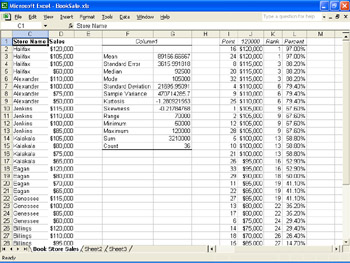
Figure 11-9: Data created by Analysis ToolPak functions run through the InsertAnalysisToolPakFunctions subroutine.

Conditionally Format Worksheet Cells

To this point, you have predominantly seen code that uses the Excel Worksheet and Range objects. To conditionally format worksheet cells programmatically, you must use the Excel FormatCondition object to both specify and apply conditional formats to cells. The following code sample applies conditional formatting to cells in the Sales column in the BookSale.xls file in the Chap11 folder.

Public Sub AddConditionalFormatting() ’ Purpose: Adds conditional formatting to the Sales column. Dim objWorksheet As Excel.Worksheet Dim objRange As Excel.Range Dim objFormatCondition1 As Excel.FormatCondition Dim objFormatCondition2 As Excel.FormatCondition ’ Select the list. Set objWorksheet = _ Excel.Application.ActiveWorkbook.Sheets(Index:="Book Store Sales") Set objRange = objWorksheet.Range(Cell1:="D2", Cell2:="D37") ’ Color the cell red if sales is less than or equal to $75,000. Set objFormatCondition1 = objRange.FormatConditions.Add _ (Type:=xlCellValue, _ Operator:=xlLessEqual, Formula1:="75000") objFormatCondition1.Interior.Color = RGB(255, 0, 0) ’ Color the cell green if sales is greater than ’ or equal to $100,000. Set objFormatCondition2 = objRange.FormatConditions.Add _ (Type:=xlCellValue, _ Operator:=xlGreaterEqual, Formula1:="100000") objFormatCondition2.Interior.Color = RGB(0, 255, 0) Set objFormatCondition2 = Nothing Set objFormatCondition1 = Nothing Set objRange = Nothing Set objWorksheet = Nothing End Sub 

To create a conditional cell format programmatically, you use the Add method of the FormatConditions collection to create an instance of a FormatCondition object. In this case, the Add method’s Type argument is set to the xlCellValue constant to specify that the conditional cell format is based on cell values. The Operator argument is set to xlLessEqual in the first condition and xlGreaterEqual in the second condition. Both xlLessEqual and xlGreaterEqual are constants. They specify that the conditional cell format represents a less- than-or-equal-to or greater-than-or-equal-to test. The Formula1 argument is set to 75000 in the first condition and 100000 in the second, specifying that cells will be tested against the $75,000 and $100,000 figures, respectively.

The Color property of the FormatCondition object’s Interior object is set to a red-green-blue combination of RGB(255, 0, 0) and RGB(0, 255, 0), respectively, to specify a red or green color.

In summary, any cell in the Sales column that is less than or equal to $75,000 will be colored red, and any cell in the Sales column that is greater than or equal to $100,000 will be colored green. The result of running the AddConditionalFormatting subroutine is shown in Figure 11-10.

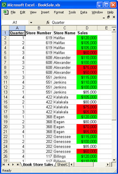
Figure 11-10: Result of running the AddConditionalFormatting subroutine.

Create PivotTable Reports and PivotChart Reports

The code required to create PivotTable reports and PivotChart reports is not significantly more difficult than the code in the Excel solutions described to this point. However, several Excel programmatic objects must be created and managed in a solution that involves data pivoting, including objects that represent the Excel workbook’s pivot cache, the PivotTable report object itself, PivotTable report fields, and an Excel Chart object that turns into a PivotChart report. The following code sample from the Chap11 folder’s BookSale.xls file shows how to work with PivotTable reports and PivotChart reports.

Public Sub CreatePivotTableAndPivotChartReport() ’ Purpose: Creates a PivotTable report and PivotChart report based on ’ the book store sales data. Dim objWorksheet As Excel.Worksheet Dim objRange As Excel.Range Dim objPivotCache As Excel.PivotCache Dim objPivotTable As Excel.PivotTable Dim objRowField As Excel.PivotField Dim objPageField As Excel.PivotField Dim objDataField As Excel.PivotField Dim objChart As Excel.Chart ’ Select the list from which to create a PivotTable report. Set objWorksheet = Excel.Application.ActiveWorkbook.Worksheets _ (Index:="Book Store Sales") Set objRange = objWorksheet.Range(Cell1:="A1", Cell2:="D37") ’ Create the PivotTable report. Set objPivotCache = Excel.Application.ActiveWorkbook.PivotCaches.Add _ (SourceType:=xlDatabase, SourceData:=objRange) Set objPivotTable = objPivotCache.CreatePivotTable _ (TableDestination:="") ’ Add the row, page, and data fields. Set objRowField = objPivotTable.PivotFields(Index:="Store Name") objRowField.Orientation = xlRowField Set objPageField = objPivotTable.PivotFields(Index:="Quarter") objPageField.Orientation = xlPageField Set objDataField = objPivotTable.PivotFields(Index:="Sales") objDataField.Orientation = xlDataField ’ Format the Sales field as currency. objDataField.NumberFormat = "$#,##0.00" ’ Create a PivotChart column-style report using the PivotTable report. Set objChart = _ Excel.Application.ActiveWorkbook.Charts.Add(Before:=objWorksheet) objChart.SetSourceData Source:=objPivotTable.TableRange2, PlotBy:=xlRows objChart.ChartType = xlColumnClustered Set objChart = Nothing Set objDataField = Nothing Set objPageField = Nothing Set objRowField = Nothing Set objPivotTable = Nothing Set objPivotCache = Nothing Set objRange = Nothing Set objWorksheet = Nothing End Sub

Here’s an explanation of the key elements of the CreatePivotTableAndPivotChartReport subroutine.

• The code calls the Add method of the Workbook object’s PivotCaches collection to add a pivot cache, which represents the in-memory cache of a workbook’s PivotTable report connections. In this instance, the Add method’s SourceType argument is set to the xlDatabase constant to specify that the PivotTable report’s data source is an internal data source. The SourceData argument specifies the list of data records on the Book Store Sales worksheet. After you programmatically create a pivot cache, you create a PivotTable report by calling the PivotCache object’s CreatePivotTable method. The TableDestination argument specifies the cell where the upper-left corner of the PivotTable will appear.

• The default Item property of the PivotTable object’s PivotFields method is called to refer to individual PivotField objects representing PivotTable fields. The objRowField, objPageField, and objDataField objects represent PivotTable report row, page, and data fields. They are added to the appropriate areas of the PivotTable report by setting the objects’ Orientation properties to the xlRowField, xlPageField, and xlDataField constants, respectively.

• The objDataField object’s NumberFormat property is set to “$#,##0.00” to specify a currency format for the sales figures. (For example, the number 1536.82 will be displayed as $1,536.82.)

• To create a linked PivotTable chart, a generic Excel chart is programmatically created when the Add method of the Excel Workbook object’s Charts collection is called. The Add method’s Before argument specifies the sheet before which the new sheet is added. In this instance, this specifies that the chart should appear on a new worksheet as the first worksheet in the Excel workbook.

• The Chart object’s SetSourceData method turns the generic Excel chart into a PivotChart report by linking the PivotTable report object to the chart object. The SetSourceData method’s Source argument is set to the PivotTable report object’s TableRange2 property, which returns all the PivotTable report’s information to the chart (the PivotTable object’s TableRange1 property doesn’t return the PivotTable report’s page fields, so it is not used in this example). The SetSourceData method’s PlotBy argument is set to the xlRows constant to indicate that the data should be plotted by rows instead of columns.

• Finally, the Chart object’s ChartType property is set to the xlColumnClustered constant to specify a clustered column chart layout.

The result of running the CreatePivotTableAndPivotChartReport subroutine is shown in Figure 11-11.

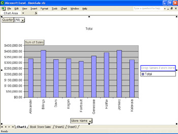
Figure 11-11: Results of running the CreatePivotTableAndPivotChartReport subroutine.

Opening and Saving XML Data in Excel

Using a program to open and save XML data in Excel is similar to opening and saving other types of data in Excel, as shown in the following two subroutines, included in the BookSale.xls file. The first subroutine opens an XML file.

Public Sub OpenAnXMLFile() ’ Purpose: Opens an XML file. ’ Change the Filename argument to match wherever you ’ store the Customers1.xml file on your computer. Application.Workbooks.OpenXML Filename:= _ "C:\Microsoft Press\Excel Data Analysis _ \Sample Files\Chap10\Customers1.xml" End Sub

In the OpenAnXMLFile subroutine, the Workbooks collection’s OpenXML method simply opens the XML data file specified in its Filename argument. (You can use the OpenXML method’s optional Stylesheets argument to specify, with either a single value or an array of values, which XSLT stylesheet processing instructions to apply to the XML file’s data before opening it in Excel.)

The following code saves data as an XML file.

Public Sub SaveXMLData() ’ Purpose: Outputs the book store sales list as XML data ’ in different XML formats. ’ Save the active workbook as an XMLSS-formatted file. Excel.ActiveWorkbook.SaveAs Filename:="C:\BookSale.xml", _ FileFormat:=xlXMLSpreadsheet Dim objWorksheet As Excel.Worksheet Dim objRange As Excel.Range ’ Select just the first 10 rows of the book store sales list. Set objWorksheet = Excel.Application.ActiveWorkbook.Sheets _ (Index:="Book Store Sales”) Set objRange = objWorksheet.Range(Cell1:="A1", Cell2:="D10”) ’ Display the results in XDR format. Debug.Print objRange.Value(xlRangeValueMSPersistXML) ’ Display the results in XMLSS format. Debug.Print objRange.Value(xlRangeValueXMLSpreadsheet) Set objRange = Nothing Set objWorksheet = Nothing End Sub

In the SaveXMLData subroutine, the Excel Workbook object’s SaveAs method saves the data at the path and file name specified by the Filename argument. To save the data using the Excel XML Spreadsheet Schema (XMLSS), the FileFormat argument is set to the constant xlXMLSpreadsheet. (There are over 40 different file formats that you can specify besides XML).

To return the results of a group of cells formatted as XML data, you can call the Range object’s Value property. Use the constant xlRangeValueMSPersistXML to return the Range object’s data formatted in the XML-Data Reduced (XDR) format, for example, if you were working with an older XML solution that requires data to be formatted in the XDR format. In most cases, however, you use the constant xlRangeValueXMLSpreadsheet to return the Range object’s data formatted in the Excel XML Spreadsheet schema (XMLSS) format.

The results of running SaveXMLData are shown in Figure 11-12 and Figure 11-13.

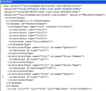
Figure 11-12: Results of running the SaveXMLData subroutine with XDR-formatted data.

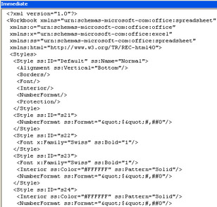
Figure 11-13: Results of running the SaveXMLData subroutine with XMLSS-formatted data.