Section 5.3. Application Design

5.3. Application Design

The application contains three worksheets. A sheet named Data holds the data. It has no formulas and no real formatting. It is just a place for the information. All the calculations are done on the Workarea sheet. It references the Data sheet, does all of the calculations, and builds named display ranges. The Display sheet uses the named ranges on Workarea, formatting, and a chart to present the results to the user. This sheet also uses controls to allow the user to interact with the application.

5.3.1. The Data Sheet

The Data sheet is shown in Figure 5-4.

Figure 5-4. The Data sheet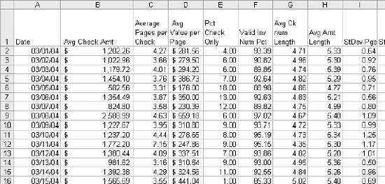

Headings are in row one. Dates go in column A and the metrics fill out the columns to the right. The sample application will handle up to 25 metrics and up to 1,000 days of data. These limits are arbitrary and can easily be increased.

Changing the data is also simple. The new data must be arranged the same way, with headings and dates. Just select and clear the entire sheet. Don't delete the columns, just clear them. Then paste your data onto the sheet starting in cell A1. The formulas on Workarea do the rest. Everything updates automatically.

5.3.2. The Workarea Sheet

All the logic and calculations are on the Workarea sheet. A few conventions are used to make this sheet easier to understand. Some ranges on this sheet are linked to the Data sheet, and they are in blue font. Named ranges used on the Display sheet have a grey background. Ranges that are used together, but not named, have a border. An example is the cells used to populate the chart. All the intermediate calculations are in column A and the results are named. Values set by controls on the Display sheet are bold and in red font.

The layout of Workarea is shown in Figure 5-5.

Item 1 is the range that populates the chart on the Display sheet. The first two columns reference the Data sheet. Item 2 is a named range called DisplayData. This data appears in the upper-left part of the Display sheet. Item 3 is also a named range. It is called ScrollArea and feeds the scrolling area on Display.

Item 4 is a range that references the column headings in row 1 of the Data sheet. It appears in the combo box on Display and allows the user to select a metric. The combo box sets the value in cell A9. The number in cell A9 is the row of the item selected. In Figure 5-5 the value is 1. This means the first item, Average Check Amount, has been selected.

Figure 5-5. Layout of Workarea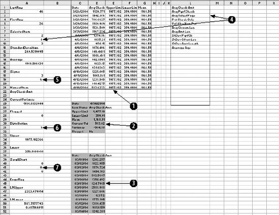

If the user changes the sigma, the spinner control sets the value in cell A19 (Item 5). The option boxes handle changes in the distribution. The option boxes both link to cell A31 (Item 6). When the first option box is checked, A31's value is 1; if the second is checked, the value is 2.

Item 7, cell A41, is set by the scroll bar control. The value is set to a number from 0 to 100, indicating how far down the scroll bar is.

The calculations are in column A. The named cells show their name above them. For example, cell A2 is named LastRow, so the cell A1 contains the name LastRow.

5.3.3. The Controls on the Display Sheet

The Display sheet contains four controls. The combo-box control lets the user select an item from a list. Controls are on the Forms toolbar . (To display the Forms toolbar, select View Toolbars.) Then check Forms.

To use a combo box, we need a list of items to select from. In the example in Figure 5-6, we start by clicking on the combo box on the toolbar (Item 1).

Figure 5-6. Setting up a combo box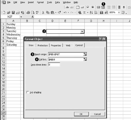

We then draw the box on the worksheet (Item 2). Use the mouse to select the location. Hold the left mouse button down and drag the mouse to indicate the size box you want. When you release the mouse button, the combo box will be there.

Right-click on the combo box and select Format Control. The Format Object box in Figure 5-6 will display. Enter the cell range to be displayed in the Input range box (Item 3). In Figure 5-6 the user will select a day of the week. The names of the days are in the range A1:A7.

Item 4 is the Cell link. When the user selects an item from the list, the combo box will put a number in this cell. The number tells which item was selected.

Figure 5-7 shows how the combo box works. When the user clicks on the box, the list is displayed. In this case Tuesday has been selected. The number 3 in cell A10 tells us the user selected the third item.

Figure 5-7. Using the combo box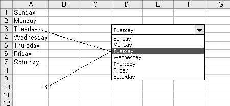

Figure 5-8 shows how the scrollbar is set up. Item 1 is the scrollbar control on the Forms toolbar. You drag and drop the control on the worksheet. In Figure 5-8 the link cell is A10. Item 2 shows how the link is set and how it works. The scrollbar is halfway down and the value in A10 is 50. In the Format Control window, the Minimum value is 0 and the Maximum is 100, so halfway is 50.

The spinner control (Item 1) in Figure 5-9 is set up like the scrollbar. They just look different. The option box (Item 2) is similar. In the project there are two option boxes, and they link to the same cell. The value in the linked cell tells which option box is selected. Excel keeps up with how many option boxes there are and only allows one of them to be selected at a time.

There are also group boxes (Item 3) on the Display sheet. They don't do anything in this application, and here they are just for looks. They are generally used to group radio button controls , and handle the logic that allows only one radio button to be checked.

5.3.4. Linking the Workarea Sheet to the Data Sheet

The Data sheet contains a lot of information, but we only use a small part of it at any given time. The user selects the column using the selector on the display sheet. The area of interest is the last 20 rows in that column. We know that the dates are in column A of Data, and we need the last 20 rows.

Figure 5-10 shows how we reference the data. LastRow, cell A2, keeps up with the last row on Data that is used. It is an array formula that multiplies the row numbers times a list of truth values (0 or 1) that are 1 for the rows that contain information. The row numbers of empty rows are multiplied by 0, so they become 0. The Maximum is the highest row that has anything in it.

Figure 5-8. Setting up and using a scrollbar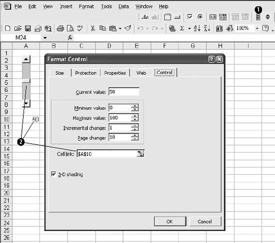

Figure 5-9. Other controls

We do not just want the last row, but the last 20 rows. The first row that we will use is 20 rows above LastRow. So, FirstRow, in cell A5, is equal to LastRow-20. These calculations on Workarea are shown in Figure 5-10.

The dates are in column C, but what about the metric? The combo box sets a value in cell A9 telling us which metric was chosen. But on the Data sheet the first column, column A, is for dates, so we have to add one to the value in A9. This gives us SelectedItem in cell A8. It is the column number of the metric we need.

The dates are referenced in column C using the INDEX function. The range is the first 1,000 rows of column A on the Data sheet. The formula in C2 uses FirstRow + ROW(A1) to reference the correct item in the range. =ROW(A1) has a value of 1. As this formula fills down, the A1 becomes A2, A3, and so on. FirstRow is deliberately set to one row above the first cell so the formula will fill down.

Figure 5-10. Connecting to the Data sheet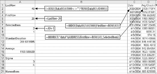

For the metrics we use the INDIRECT function because it allows us to reference both row and column. The formula in D2 uses ADDRESS to build the reference and INDIRECT to get the value. The parameters for the ADDRESS function are row and column number. The row number is calculated just like the INDEX formula in column C. The column number is SelectedItem.

5.3.4.1. Calculations on the Workarea Sheet

The next part of Workarea is shown in Figure 5-11.

We use the numbers in the range D2:D20 to set the control limits. The value in D21 is the current value, the one we are checking. Therefore, we do not use it to set the limits.

The formula in A12 returns the standard deviation of the range. In A15 we get the average.

Cell A19 is set by the spinner control and can be from 0 to 12 in increments of 1. We are going to let the user select a sigma in the range 0 to 6 in increments of one half. The formula in A18 divides the set value by 2 and returns the sigma used in the calculations.

Cell D21 contains the current value. The named value Average is the average of the last 19 days. CurrentVariance is the difference between D21 and Average. This part of Workarea is in Figure 5-12.

The named values Upper and Lower are the control limits. In Figure 5-12 cell A28 (named Flagged) checks the current value of cell D21. If the value is higher than Upper or Lower then the value is set to 1. This indicates the current value is out of the control limits.

Figure 5-11. Calculations on Workarea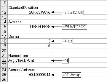

The calculation of Upper depends on the distribution selection. If it is normal, the named value Distribution is 1. In that case Upper is =Average + (Sigma * StandardDeviation), which is the named value NUpper. Otherwise it is based on the log normal distribution. The named value LNUpper has the value. A similar technique is used for Lower. It is either based on the Average, Sigma, and Standard Deviation, NLower, or it uses the log normal calculation LNLower.

The scrolling area on Display is controlled by the value ScrollStart. It is the row number of the first row of Data shown in the scrolling area. When the user moves the scrollbar, a value from 0 to 100 is set in cell A41. This value tells how far down the scrollbar is. The formula in cell A42 uses this value to decide what row on Data should be the first of the 15 rows of the scroll area.

The scrolling calculations work from the bottom up, so it is possible to get a row number that is less than 1. That would cause an error, and the formula in cell A40 takes the maximum of the value in A42 and 1. 1 is subtracted from the answer to simplify the formulas in Scrollarea.

Cell A51 contains an array formula that calculates the standard deviation based on the log of the values in D2:D20 and multiplies the answer by sigma. This value is added to the log of the average to obtain log normal upper limit in A47 (LNUpper). The EXP function is applied to the result turning it back into a value for the chart. If the value in A51 is an error, there are values in the range D2:D20 that are not positive real numbers and the Log cannot be taken. If this is the case and log normal distribution is selected, an error message is built in cell A45 (ErrorFlag). In an error condition, the normal distribution limit is used.

Figure 5-12. More calculations on Workarea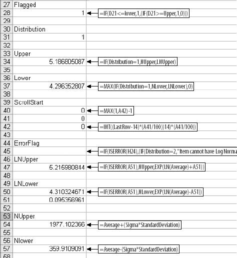

The calculations in A50 (LNLower) are for the lower log normal limit. They are the same as A47 except the value in A51 is subtracted from the average.

The named values NUpper and NLower are in cells A54 and A57. They are the upper and lower control limits based on a normal distribution.

Isolating the calculations keeps the application simple. There are several things going on with the control limits, but each part of Workarea only does one thing. It is important to break multi-step processes down to basic elements. If you can understand how each step works, you can build the entire process.

5.3.5. The Display Sheet

The most complex part of the Display sheet is the scroll.

5.3.5.1. The scroll

Figure 5-13 shows how the scroll area works. The data is on the Data sheet. The dates (Item 1) are always in column A. The metric to be displayed is in one of the other columns. Since the dates are in A, the formula in item 3 can use the INDEX function. ScrollStart tells which row to start with, and adding =ROW(A1) makes it possible to fill the formula down. The metric in item 2 is the one to be displayed. The column is identified by SelectedItem and the row by ScrollStart in the formula shown in item 4. This range is named ScrollArea.

On the Display sheet, the scroll (Item 5) contains the array formula {=ScrollArea}. The scroll is formatted using patterns and borders. The scrollbar is linked to cell A41 (Item 6) on Workarea, completing the connection.

Figure 5-13. Building the scroll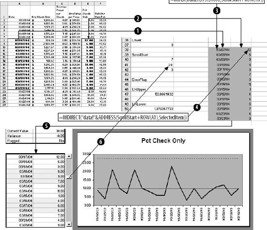

5.3.5.2. Other parts of the Display sheet

The chart area is completed using named values shown in Figure 5-14.

Figure 5-14. Completing the chart area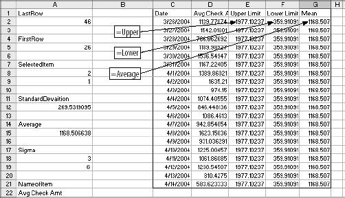

Columns E, F, and G are used to draw lines on the chart showing the control limits and the mean. Using this range, a line chart is inserted on Display. The other piece of the Display sheet is the area shown in Figure 5-15.

Figure 5-15. Data display area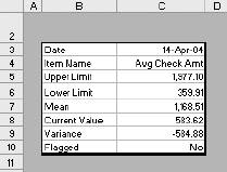

This links to the named range DisplayData on the Workarea sheet. Displayarea, C25:D32, uses named values to arrange the data for Display. The array formula for Display is {=DisplayData}.