Section 1.1. Array Formulas

1.1. Array Formulas

Excel array formulas give you the ability to work on ranges of cells all at once. Suppose we have a list of numbers, and we want to know the average amount of change from one number to the next. This situation is illustrated in Figure 1-1.

The normal way to approach a problem like this is to add a new column with an intermediate calculation. In cell B2 we calculate the difference between A2 and A1. Then we fill this formula down to cell B10. In cell B12 we simply take the average.

With an array formula we can get the same answer using only one cell. The formula in B15 is:

 =AVERAGE(A2:A10-A1:A9)

This makes sense. We want the average of the differences, and that is what the formula is asking for. However, this returns a value error! The error appears because we need to enter the formula in a special way that tells Excel the formula applies to the ranges and not to individual cells.

This is done by pressing Ctrl-Shift-Enter, all at the same time while entering the formula. Excel then displays the formula in brackets, as shown in cell B17:

 {=AVERAGE(A2:A10-A1:A9)}

Figure 1-1. Using an array formula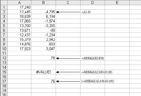

The values returned in cells B12 and B17 are the same. Excel does all of the intermediate calculations and returns the result.

Array formulas save space on the worksheet; often whole columns of formulas can be eliminated. By reducing visual complexity, they make things easier to understand, and can speed up sheet recalculation.

Array formulas can also contain truth values . Excel considers true to be a binary 1 and false to be a binary 0, and sometimes this can be helpful.

In Figure 1-2 we need to find the average of the odd numbers in the list.

In the non-array approach, we would start by identifying the odd values. If a number divided by two is not equal to the integer value of itself divided by two, it is odd. The formula in cell B1 is:

 =A1/2<>INT(A1/2)

This fills down to B10 and returns a value of true (binary 1) if the number is odd and false (binary 0) if it is even.

In cell C1, this is the formula:

 =B1*A1

If B1 is false, it equals zero and the returned value will be zero. But if the value is true, as it will be if A1 is odd, it is a one and the returned value will be equal to A1.

In column D we do the same thing, but this time we multiply by one using this formula:

Figure 1-2. Averaging the odd numbers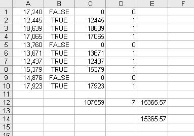

 =B1*1

This is useful because many Excel functions do not recognize binary trUE and FALSE values. This simple formula converts the binary value into a number that can be used in other calculations.

We could avoid this issue, and the need for the formulas in the D column in Figure 1-2, by using the COUNTIF function. But it is still important to know how to get truth values into other calculations.

The formulas in C12 and D12 take the sum of the cells above, and in cell E12 we divide C12 by D12. Since C12 has the sum of the odd values and D12 has the count, this gives the average.

We can get the same result with this array formula:

 {=(SUM((A1:A10/2<>INT(A1:A10/2))*A1:A10))/(SUM((A1:A10/2<>INT(A1:A10/2))*1))}

It does the work of two columns, two sums, and a division function. And, it does it exactly the same way. The difference is that the formula is built on ranges, not individual cells. All of the same logical steps are in the array formula.