Backpropagation Learning | Visual Basic Developers Guide to ASP and IIS: Build Powerful Server-Side Web Applications with Visual Basic. (Visual Basic Developers Guides)

Backward error propagation, or simply backpropagation, is the most popular learning algorithm for connectionist learning. As the name implies, an error in the output node is corrected by back propagating this error by adjusting weights through the hidden layer and back to the input layer. While relatively simple, convergence can take some time depending upon the allowable error in the output.

Backpropagation Algorithm

The algorithm begins with the assignment of randomly generated weights for the multi-layer, feed-forward network. The following process is then repeated until the mean-squared error (MSE) of the output is sufficiently small:

Take a training example E with its associated correct response C.
Compute the forward propagation of E through the network (compute the weighted sums of the network, S _i , and the activations, u _i , for every cell ).
Starting at the outputs, make a backward pass through the output and intermediate cells , computing the error values (Equations 5.3 and 5.4):

(5.3)

(5.4)

(Note that m denotes all cells connected to the hidden node, w is the given weight vector and u is the activation).

Finally, the weights within the network are updated as follows (Equations 5.5 and 5.6):

(5.5)

(5.6)

where represents the learning rate (or step size ). This small value limits the change that may occur during each step.

Tip	The parameter can be tuned to determine how quickly the backpropagation algorithm converges toward a solution. It's best to start with a small value (0.1) to test and then slowly increment.

The forward pass through the network computes the cell activations and an output. The backward pass computes the gradient (with respect to the given example). The weights are then updated so that the error is minimized for the given example. The learning rate minimizes the amount of change that may take place for the weights. While it may take longer for a smaller learning rate to converge, we minimize overshooting our target. If the learning rate is set too high, the network may never converge.

We'll see the actual code that's required to implement the functions above, listed with the numerical steps for the backpropagation algorithm as shown above.

Backpropagation Example

Let's now look at an example of backpropagation at work. Consider the network shown in Figure 5.7.

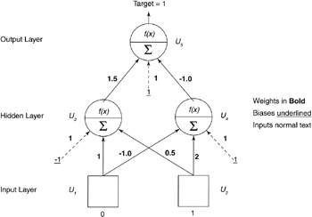
Figure 5.7: Numerical backpropagation example.

The Feed-forward Pass

First, we feed forward the inputs through the network. Let's look at the values for the hidden layer:

u ₃ = f ( w _3,1 u ₁ + w _3,2 u ₂ + w _b *bias )
u ₃ = f (1*0 + 0.5*1 + 1*1) = f (1.5)
u ₃ = 0.81757
u ₄ = f ( w _4,1 u ₁ + w _4,2 u ₂ + w _b *bias )
u ₄ = f (-1*0 + 2*1 + 1*1) = f (3)
u ₄ = 0.952574

Recall that f ( x ) is our activation function, the sigmoid function (Equation 5.7):

(5.7)

Our inputs have now been propagated to the hidden layer; the final step is to feed the hidden layer values forward to the output layer to calculate the output of the network.

u ₅ = f ( w _5,3 u ₃ + w _5,4 u4 + w _b *bias )
u ₅ = f (1.5*0.81757+ -1.0*0.952574+ 1*1) = f (1.2195)
u ₅ = 0.78139

Our target for the neural network was 1.0; the actual value computed by the network was 0.78139. This isn't too bad, but by applying the backpropagation algorithm to the network, we can reduce the error.

The mean squared error is typically used to quantify the error of the network. For a single node, this is defined as Equation 5.8:

(5.8)

Therefore, our error is:

err = 0.5 * (1.0 - 0.78139) ² = 0.023895

The Error Backward Propagation Pass

Now let's apply backpropagation, starting with determining the error of the output node and the hidden nodes. Using Equation 5.1, we calculate the output node error:

_o = (1.0 - 0.78139) * 0.78139 * (1.0 - 0.78139)
_o = 0.0373

Now we calculate the error for both hidden nodes. We use the derivative of our sigmoidal equation (Equation 5.5), which is shown as Equation 5.9.

(5.9)

Using Equation 5.2, we now calculate the errors for the hidden nodes:

_u4 = ( _o * w _5,4 ) *u ₄ * (1.0 - u ₄ )
_u4 = (0.0373 * -1.0) * 0.952574 * (1.0 - 0.952574)
_u4 = -0.0016851
_u3 = ( _o * w _5,3 ) *u ₃ * (1.0 - u ₃ )
_u3 = (0.0373 * 1.5) * 0.81757 * (1.0 - 0.81757)
_u3 = 0.0083449

Adjusting the Connection Weights

Now that we have the error values for the output and hidden layers , we can use Equations 5.3 and 5.4 to adjust the weights. We'll use a learning rate ( ) of 0.5. First, we'll update the weights that connect our output layer to the hidden layer.

w* _i,j = w _i,j + _o u _i
w _5,4 = w _5,4 + ( * 0.0373 * u ₄ )
w _5,4 = -1 + (0.5 * 0.0373 * 0.952574)
w _5,4 = -0.9822
w _5,3 = w5,3 + ( * 0.0373 * u ₃ )
w _5,3 = 1.5 + (0.5 * 0.0373 * 0.81757)
w _5,3 = 1.51525

Now, let's update the output cell bias:

w _5,b = w _5,b + ( * 0.0373 * bias ₅ )
w _5,b = 1 + (0.5 * 0.0373 * 1)
w _5,b = 1.01865

In the case of w _5,4 , the weight was decreased where for w _5,3 the weight was increased. Our bias was updated for greater excitation . Now we'll show the adjustment of the hidden weights (for the input to hidden cells).

w* _i,j = w _i,j + _i u _i
w _4,2 = w _4,2 + ( * -0.0016851 * u ₂ )
w _4,2 = 2 + (0.5 * -0.0016851 * 1)
w _4,2 = 1.99916
w _4,1 = w _4,1 + ( * -0.0016851 * u ₁ )
w _4,1 = -1 + (0.5 * -0.0016851 * 0)
w _4,1 = -1.0
w _3,2 = w _3,2 + ( * 0.0083449 * u ₂ )
w _3,2 = 0.5 + (0.5 * 0.0083449 * 1)
w _3,2 = 0.50417
w _3,1 = w _3,1 + ( * 0.0083449 * u ₁ )
w _3,1 = 1.0 + (0.5 * 0.0083449 * 0)
w _3,1 = 1.0

The final step is to update the cell biases:

w _4,b = w _4,b + ( * -0.0016851 * bias ₄ )
w _4,b = 1.0 + (0.5 * -0.0016851 * 1)
w _4,b = 0.99915
w _3,b = w _3,b + ( * 0.0083449 * bias ₃ )
w _3,b = 1.0 + (0.5 * 0.0083449 * 1)
w _3,b = 1.00417

That completes the updates of our weights for the current training example. To verify that the algorithm is genuinely reducing the error in the output, we'll run the feed-forward algorithm one more time.

u ₃ = f ( w _3,1 u ₁ + w _3,2 u ₂ + w _b *bias )
u ₃ = f (1*0 + 0.50417*1 + 1.00417*1) = f (1.50834)
u ₃ = 0.8188
u ₄ = f ( w _4,1 u ₁ + w _4,2 u ₂ + w _b *bias )
u ₄ = f (-1*0 + 1.99916*1 + 0.99915*1) = f (2.99831)
u ₄ = 0.952497
u ₅ = f ( w _5,3 u ₃ + w _5,4 u ₄ + w _b *bias )
u ₅ = f (1.51525*0.8188+ -0.9822*0.952497 + 1.01865*1) = f (1.32379)
u ₅ = 0.7898
err = 0.5 * (1.0 - 0.7898) ² = 0.022

Recall that the initial error of this network was 0.023895. Our current error is 0.022, which means that this single iteration of the backpropagation algorithm reduced the mean squared error by 0.001895.