Multiple-Layer Networks

Multiple-Layer Networks

Multiple-layer networks permit more complex, non-linear relationships of input data to output results. From Figure 5.4, we can see that the multiple-layer network is made up of an input layer, an intermediate or hidden layer, and an output layer. The input layer simply represents the inputs to the network, and is not composed of cells (neurons) in the traditional sense. The naming of cells , chosen for this example, gives each cell a u _n identifier. The two input cells are named [ u ₁ , u ₂ ], two hidden cells [ u ₃ , u ₄ ], and one output cell [ u ₅ ]. Identifying connections within the network is standardized as w _3,1 , and represents the weighted connection between u ₃ and u ₁ .

While input cells ( u ₁ and u ₂ ) simply provide an input value to the network, hidden and output cells represent a function (recall Equation 5.1). The result of the sum of products is fed through a squashing function (typically a sigmoid), which results in the output of the cell. The sigmoid function is shown in Figure 5.5.

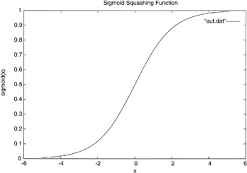
Figure 5.5: The sigmoid (squashing) activation function.

Let's now look at the complete picture of a neural network cell. In Figure 5.6, we see the output cell from the network shown in Figure 5.4. The output cell u ₅ is fed by the two hidden cells, u ₃ and u ₄ , through weights w _5,3 and w _5,4 respectively.

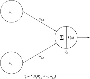
Figure 5.6: Hidden and output layers of a sample neural network.

One important note here is that the sigmoid function should be applied to the hidden nodes in the sample network in Figure 5.6, but they are omitted in this case to illustrate the output layer processing only. The equation in Figure 5.6 illustrates the sum of products of the inputs from the hidden layer with the connection weights. The f ( x ) function represents the sigmoid applied to the result.

In a network with a hidden layer and an output layer, the hidden layer is computed first and then the results of the hidden layer are used to compute the output layer.