Issues with Two or More Data Fields

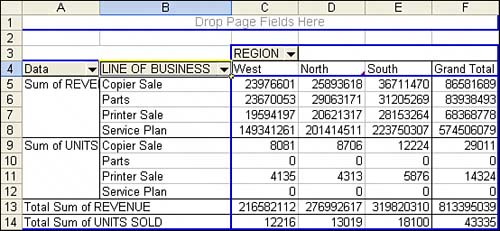
So far, you have built some powerful summary reports, but you've touched only a portion of the powerful features available in pivot tables. The prior example produced a report but had only one data field.

It is possible to have multiple fields in a pivot report.

The data in this example includes not just revenue, but also units. The CFO will probably appreciate a report by product that shows quantity sold, revenue, and average price.

When you have two or more data fields, you have a choice of placing the data fields in one of four locations. By default, Excel builds the pivot report with the data field as the innermost row field. It is often preferable to have the data field as the outermost row field or as a column field.

When a pivot table is going to have more that one data field, you have a virtual field named Data. Where you place the Data field in the .AddFields method determines which view of the data you get.

The default setup, with the data fields arranged as the innermost row field, as shown in Figure 12.11, would have this AddFields line:

 PT.AddFields RowFields:=Array("Line of Business", "Data") 

Figure 12.11. The default pivot table report has the multiple data fields as the innermost row field.

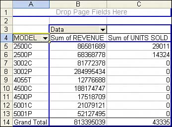
The view shown in Figure 12.12 would use this code:

 PT.AddFields RowFields:=Array("Data", "Line of Business") 

Figure 12.12. By moving the Data field to the first row field, you can obtain this view of the multiple data fields.

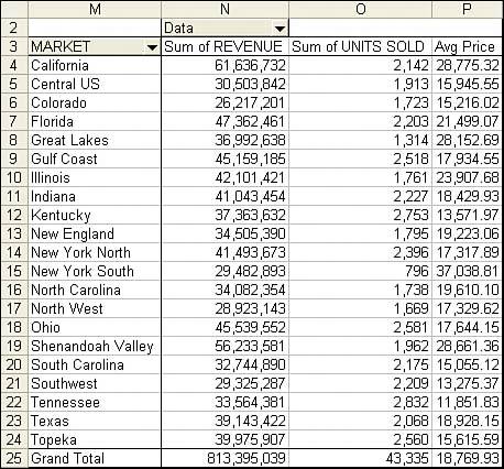
The view that you need for this report would have Data as a column field:

 PT.AddFields RowFields:="Model", ColumnFields:="Data" 

After adding a column field called Data, you would then go on to define two data fields:

 ' Set up the data fields With PT.PivotFields("Revenue")     .Orientation = xlDataField     .Function = xlSum     .Position = 1     .NumberFormat = "#,##0" End With With PT.PivotFields("Units Sold")     .Orientation = xlDataField     .Function = xlSum     .Position = 2     .NumberFormat = "#,##0" End With 

Calculated Data Fields

Pivot tables offer two types of formulas. The most useful type defines a formula for a calculated field. This adds a new field to the pivot table. Calculations for calculated fields are always done at the summary level. If you define a calculated field for average price as Revenue divided by Units Sold, Excel first adds up the total revenue and the total quantity, and then it does the division of these totals to get the result. In many cases, this is exactly what you need. If your calculation does not follow the associative law of mathematics, it might not work as you expect.

To set up a calculated field, use the Add method with the CalculatedFields object. You have to specify a field name and a formula. Note that if you create a field called Average Price, the default pivot table produces a field called Sum of Average Price. This is misleading and downright silly. What you have is actually the average of the sums of prices. The solution is to use the Name property when defining the data field to replace Sum of Average Price with something such as Avg Price. Note that this name must be different from the name for the calculated field.

Listing 12.2 produces the report shown in Figure 12.13.

Listing 12.2. Code That Calculates an Average Price Field as a Second Data Field

 Sub TwoDataFields()     Dim WSD As Worksheet     Dim PTCache As PivotCache     Dim PT As PivotTable     Dim PRange As Range     Dim FinalRow As Long     Set WSD = Worksheets("PivotTable")     Dim WSR As Worksheet     Dim WBO As Workbook     Dim WBN As Workbook     Set WBO = ActiveWorkbook     ' Delete any prior pivot tables     For Each PT In WSD.PivotTables         PT.TableRange2.Clear     Next PT     ' Define input area and set up a Pivot Cache     FinalRow = WSD.Cells(Application.Rows.Count, 1).End(xlUp).Row     FinalCol = WSD.Cells(1, Application.Columns.Count). _         End(xlToLeft).Column     Set PRange = WSD.Cells(1, 1).Resize(FinalRow, FinalCol)     Set PTCache = ActiveWorkbook.PivotCaches.Add(SourceType:= _         xlDatabase, SourceData:=PRange.Address)     ' Create the Pivot Table from the Pivot Cache     Set PT = PTCache.CreatePivotTable(TableDestination:=WSD. _         Cells(2, FinalCol + 2), TableName:="PivotTable1")     ' Turn off updating while building the table     PT.ManualUpdate = True     ' Set up the row fields     PT.AddFields RowFields:="Market", ColumnFields:="Data"     ' Define Calculated Fields     PT.CalculatedFields.Add Name:="AveragePrice", Formula:="=Revenue/Units Sold"     ' Set up the data fields     With PT.PivotFields("Revenue")         .Orientation = xlDataField         .Function = xlSum         .Position = 1         .NumberFormat = "#,##0"     End With     With PT.PivotFields("Units Sold")         .Orientation = xlDataField         .Function = xlSum         .Position = 2         .NumberFormat = "#,##0"     End With     With PT.PivotFields("AveragePrice")         .Orientation = xlDataField         .Function = xlSum         .Position = 3         .NumberFormat = "#,##0.00"         .Name = "Avg Price"     End With     ' Ensure that you get zeroes instead of blanks in the data area     PT.NullString = "0"     ' Calc the pivot table     PT.ManualUpdate = False     PT.ManualUpdate = True End Sub 

Figure 12.13. The virtual "Data" dimension contains two fields from your dataset plus a calculation. It is shown along the column area of the report.

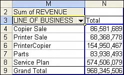
Calculated Items

Say that in your company the vice president of sales is responsible for copier sales and printer sales. The idea behind a calculated item is that you can define a new item along the Line of Business field to calculate the total of copier sales and printer sales. Listing 12.3 produces the report shown in Figure 12.14.

Listing 12.3. Code That Adds a New Item Along the Line of Business Dimension

 Sub CalcItemsProblem()     Dim WSD As Worksheet     Dim PTCache As PivotCache     Dim PT As PivotTable     Dim PRange As Range     Dim FinalRow As Long     Set WSD = Worksheets("PivotTable")     Dim WSR As Worksheet     ' Delete any prior pivot tables     For Each PT In WSD.PivotTables         PT.TableRange2.Clear     Next PT     ' Define input area and set up a Pivot Cache     FinalRow = WSD.Cells(Application.Rows.Count, 1).End(xlUp).Row     FinalCol = WSD.Cells(1, Application.Columns.Count). _         End(xlToLeft).Column     Set PRange = WSD.Cells(1, 1).Resize(FinalRow, FinalCol)     Set PTCache = ActiveWorkbook.PivotCaches.Add(SourceType:= _         xlDatabase, SourceData:=PRange.Address)     ' Create the Pivot Table from the Pivot Cache     Set PT = PTCache.CreatePivotTable(TableDestination:=WSD. _         Cells(2, FinalCol + 2), TableName:="PivotTable1")     ' Turn off updating while building the table     PT.ManualUpdate = True     ' Set up the row fields     PT.AddFields RowFields:="Line of Business"     ' Define calculated item along the product dimension     PT.PivotFields("Line of Business").CalculatedItems _         .Add "PrinterCopier", "='Copier Sale'+'Printer Sale'"     ' Resequence so that the report has printers and copiers first     PT.PivotFields("Line of Business"). _         PivotItems("Copier Sale").Position = 1     PT.PivotFields("Line of Business"). _         PivotItems("Printer Sale").Position = 2     PT.PivotFields("Line of Business"). _         PivotItems("PrinterCopier").Position = 3     ' Set up the data fields     With PT.PivotFields("Revenue")         .Orientation = xlDataField         .Function = xlSum         .Position = 1         .NumberFormat = "#,##0"     End With     ' Ensure that you get zeroes instead of blanks in the data area     PT.NullString = "0"     ' Calc the pivot table     PT.ManualUpdate = False     PT.ManualUpdate = True End Sub 

Figure 12.14. Unless you love restating numbers to the SEC, avoid using calculated items.

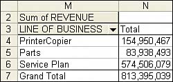
Look closely at the results shown in Figure 12.14. The calculation for PrinterCopier is correct. PrinterCopier is a total of Printers + Copiers. Some quick math confirms that 86 million + 68 million is about 154 million. However, the grand total should be 154 million + 83 million + 574 million, or about 811 million. Instead, Excel gives you a grand total of $968 million. The total revenue for the company just increased by $150 million. Excel gives the wrong grand total when a field contains both regular and calculated items. The only plausible method for dealing with this is to attempt to hide the products that make up PrinterCopier. The results are shown in Figure 12.15:

 With PT.PivotFields("Line of Business")     .PivotItems("Copier Sale").Visible = False     .PivotItems("Printer Sale").Visible = False End With 

Figure 12.15. After the components that make up the calculated PrinterCopier item are hidden, the total revenue for the company is again correct. However, it would be easier to add a new field to the original data with a Responsibility field.