Summarize Date Fields with Grouping

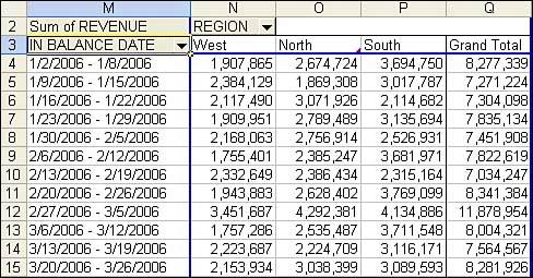
With transactional data, you will often find your date-based summaries having one row per day. Although daily data might be useful to a plant manager, many people in the company want to see totals by month or quarter and year.

The great news is that Excel handles the summarization of dates in a pivot table with ease. For anyone who has ever had to use the arcane formula =A2+1-Day(A2) to change daily dates into monthly dates, you will appreciate the ease with which you can group transactional data into months or quarters.

Creating a group with VBA is a bit quirky. The .Group method can be applied to only a single cell in the pivot table, and that cell must contain a date or the Date field label. This is the first example in this chapter where you must allow VBA to calculate an intermediate pivot table result.

You must define a pivot table with In Balance Date in the row field. Turn off ManualCalculation to allow the Date field to be drawn. You can then use the LabelRange property to locate the date label and group from there. Figure 12.16 shows the result of Listing 12.4.

Listing 12.4. Code That Uses the Group Feature to Roll Daily Dates Up to Monthly Dates

 Sub ReportByMonth()     Dim WSD As Worksheet     Dim PTCache As PivotCache     Dim PT As PivotTable     Dim PRange As Range     Dim FinalRow As Long     Set WSD = Worksheets("PivotTable")     Dim WSR As Worksheet     ' Delete any prior pivot tables     For Each PT In WSD.PivotTables         PT.TableRange2.Clear     Next PT     ' Define input area and set up a Pivot Cache     FinalRow = WSD.Cells(Application.Rows.Count, 1).End(xlUp).Row     FinalCol = WSD.Cells(1, Application.Columns.Count). _         End(xlToLeft).Column     Set PRange = WSD.Cells(1, 1).Resize(FinalRow, FinalCol)     Set PTCache = ActiveWorkbook.PivotCaches.Add(SourceType:= _         xlDatabase, SourceData:=PRange.Address)     ' Create the Pivot Table from the Pivot Cache     Set PT = PTCache.CreatePivotTable(TableDestination:=WSD. _         Cells(2, FinalCol + 2), TableName:="PivotTable1")     ' Turn off updating while building the table     PT.ManualUpdate = True     ' Set up the row fields     PT.AddFields RowFields:="In Balance Date", ColumnFields:="Region"     ' Set up the data fields     With PT.PivotFields("Revenue")         .Orientation = xlDataField         .Function = xlSum         .Position = 1         .NumberFormat = "#,##0"     End With     ' Ensure that you get zeroes instead of blanks in the data area     PT.NullString = "0"     ' Calc the pivot table to allow the date label to be drawn     PT.ManualUpdate = False     PT.ManualUpdate = True     ' Group ShipDate by Month, Quarter, Year     PT.PivotFields("In Balance Date").LabelRange.Group Start:=True, _         End:=True, Periods:= _         Array(False, False, False, False, True, True, True)     ' Calc the pivot table     PT.ManualUpdate = False     PT.ManualUpdate = True End Sub 

Figure 12.16. The In Balance Date field is now composed of three fields in the pivot table, representing year, quarter, and month.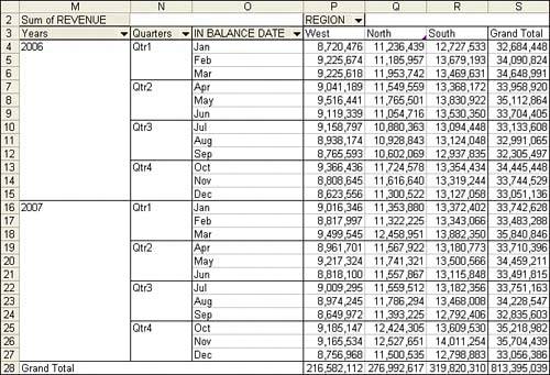

Group by Week

You probably noticed that Excel allows you to group by day, month, quarter, and year. There is no standard grouping for week. You can, however, define a group that bunches up groups of seven days.

By default Excel starts the week based on the first date found in the data. This means that the default week would run from Tuesday January 1, 2006 through Monday December 31, 2007. You can override this by changing the Start parameter from true to an actual date. Use the WeekDay function to determine how many days to adjust the start date.

There is one limitation to grouping by week. When you group by week, you cannot also group by any other measure. It is not valid to group by week and quarter.

Listing 12.5 creates the report shown in Figure 12.17.

Listing 12.5. The Code Used to Group by Week Must Figure Out the Monday Nearest the Start ofYour Data

 Sub ReportByWeek()     Dim WSD As Worksheet     Dim PTCache As PivotCache     Dim PT As PivotTable     Dim PRange As Range     Dim FinalRow As Long     Set WSD = Worksheets("PivotTable")     Dim WSR As Worksheet     ' Delete any prior pivot tables     For Each PT In WSD.PivotTables         PT.TableRange2.Clear     Next PT     ' Define input area and set up a Pivot Cache     FinalRow = WSD.Cells(Application.Rows.Count, 1).End(xlUp).Row     FinalCol = WSD.Cells(1, Application.Columns.Count). _         End(xlToLeft).Column     Set PRange = WSD.Cells(1, 1).Resize(FinalRow, FinalCol)     Set PTCache = ActiveWorkbook.PivotCaches.Add(SourceType:= _         xlDatabase, SourceData:=PRange.Address)     ' Create the Pivot Table from the Pivot Cache     Set PT = PTCache.CreatePivotTable(TableDestination:=WSD. _         Cells(2, FinalCol + 2), TableName:="PivotTable1")     ' Turn off updating while building the table     PT.ManualUpdate = True     ' Set up the row fields     PT.AddFields RowFields:="In Balance Date", ColumnFields:="Region"     ' Set up the data fields     With PT.PivotFields("Revenue")         .Orientation = xlDataField         .Function = xlSum         .Position = 1         .NumberFormat = "#,##0"     End With     ' Ensure that you get zeroes instead of blanks in the data area     PT.NullString = "0"     ' Calc the pivot table to allow the date label to be drawn     PT.ManualUpdate = False     PT.ManualUpdate = True     ' Group Date by Week.     'Figure out the first Monday before the minimum date     FirstDate = PT.PivotFields("In Balance Date").LabelRange. _         Offset(1, 0).Value     WhichDay = Weekday(FirstDate, 3)     StartDate = FirstDate - WhichDay     PT.PivotFields("In Balance Date").LabelRange.Group _         Start:=StartDate, End:=True, By:=7, _         Periods:=Array(False, False, False, True, False, False, False)     ' Calc the pivot table     PT.ManualUpdate = False     PT.ManualUpdate = True End Sub 

Figure 12.17. Use the Number of Days setting to group by week.