Handle Additional Annoyances

You've reached the end of the adjustments that you can make to the pivot table. To achieve the final report, you have to make the remaining adjustments after converting the pivot table to regular data.

Figure 12.8 shows the pivot table with all the adjustments described in the previous sections made and with PT.TableRange2 selected.

Figure 12.8. It took less than one second and 30 lines of code to get 90% of the way to the final report. To solve the last five annoying problems, you have to change this data from a pivot table to regular data.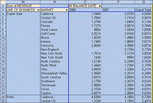

New Workbook to Hold the Report

Say that you want to build the report in a new workbook so that it can be easily mailed to the product managers. This is fairly easy to do. To make the code more portable, assign object variables to the original workbook, the new workbook, and the first worksheet in the new workbook. At the top of the procedure, add these statements:

 Dim WSR As Worksheet Dim WBO As Workbook Dim WBN As Workbook Set WBO = ActiveWorkbook Set WSD = Worksheets("Pivot Table") 

After the pivot table has been successfully created, build a blank Report workbook with this code:

 ' Create a New Blank Workbook with one Worksheet Set WBN = Workbooks.Add(xlWorksheet) Set WSR = WBN.Worksheets(1) WSR.Name = "Report" ' Set up Title for Report With WSR.Range("A1")     .Value = "Revenue by Market and Year"     .Font.Size = 14 End With 

Summary on a Blank Report Worksheet

Imagine that you have submitted the pivot table in Figure 12.8, and your manager hates the borders, hates the title, and hates the words "Line of Business" in cell O2. You can solve all three of these problems by excluding the first row(s) of PT.TableRange2 from the .Copy method and then using PasteSpecial(xlPasteValuesAndNumberFormats) to copy the data to the report sheet.

CAUTION

In Excel 2000 and earlier, xlPasteValuesAndNumberFormats was not available. You would have to Paste Special twice: once as xlPasteValues and once as xlPasteFormats.

In the current example, the .TableRange2 property includes only one row to eliminate, row 2, as shown in Figure 12.8. If you had a more complex pivot table with several column fields and/or one or more page fields, you would have to eliminate more than just the first row of the report. It helps to run your macro to this point, look at the result, and figure out how many rows you need to delete. You can effectively not copy these rows to the report by using the Offset property. Copy the TableRange2 property, offset by one row. Purists will note that this code does copy one extra blank row from below the pivot table, but this really does not matter, because the row is blank. After doing the copy, you can erase the original pivot table and destroy the pivot cache:

 ' Copy the Pivot Table data to row 3 of the Report sheet ' Use Offset to eliminate the title row of the pivot table PT.TableRange2.Offset(1, 0).Copy WSR. Range("A3").PasteSpecial Paste:=xlPasteValuesAndNumberFormats PT.TableRange2.Clear Set PTCache = Nothing 

Note that you used the Paste Special option to paste just values and number formats. This gets rid of both borders and the pivot nature of the table. You might be tempted to use the All Except Borders option under Paste, but this keeps the data in a pivot table, and you won't be able to insert new rows in the middle of the data.

Fill Outline View

The report is almost complete. You are nearly a Data, Subtotals command away from having everything you need. Before you can use the Subtotals command, however, you need to fill in all the blank cells in the outline view of column A.

Fixing the Outline view requires just a few obscure steps. Here are the steps in the user interface:

1.	Select all the cells in column A that make up the report.
2.	Select Edit, GoTo to bring up the GoTo dialog box. Click the Special button to bring up the GoTo Special dialog box. Select Blanks to select only the blank cells.
3.	Enter an R1C1-style formula to fill the blank with the cell above it. This formula is =R[1]C. In the user interface you would type an equals sign, press the up-arrow key, and then press Ctrl+Enter.
4.	Reselect all the cells in column A that make up the report. This is necessary because the Paste Special step cannot work with noncontiguous selections.
5.	Copy the formulas in column A and convert them to values by using the Values option in the Paste Special dialog box.

Fixing the Outline view in VBA requires fewer steps. The equivalent VBA logic is shown here:

1.	Find the last row of the report.
2.	Enter the formula =R[-1]C in the blank cells in A.
3.	Change those formulas to values.

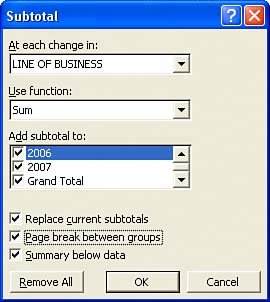
The code to do this follows:

 Dim FinalReportRow as Long     ' Fill in the Outline view in column A     ' Look for last row in column B since many rows     ' in column A are blank FinalReportRow = WSR.Range("B65536").End(xlUp).Row With Range("A3").Resize(FinalReportRow - 2, 1)     With .SpecialCells(xlCellTypeBlanks)         .FormulaR1C1 = "=R[-1]C"     End With     .Value = .Value End With 

Final Formatting

The last steps for the report involve some basic formatting tasks and then adding the sub totals. You can bold and right-justify the headings in row 3. Set rows 13 up so that the top three rows print on each page:

 ' Do some basic formatting ' Autofit columns, bold the headings, right-align Selection.Columns.AutoFit Range("A3").EntireRow.Font.Bold = True Range("A3").EntireRow.HorizontalAlignment = xlRight Range("A3:B3").HorizontalAlignment = xlLeft ' Repeat rows 1-3 at the top of each page WSR.PageSetup.PrintTitleRows = "$1:$3" 

Add Subtotals

Automatic subtotals are a powerful feature found on the Data menu. Figure 12.9 shows the Subtotal dialog box. Note the option Page Break Between Groups.

Figure 12.9. Use automatic subtotals because doing so enables you to add a page break after each product. This ensures that each product manager has a clean report with only his or her product on it.

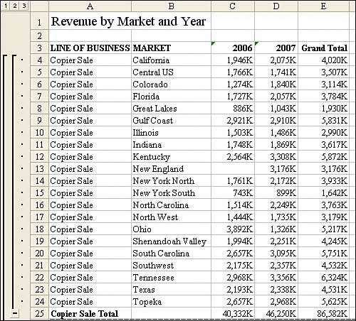
If you were sure that you would always have two years and a total, the code to add subtotals for each Line of Business group would be the following:

 ' Add Subtotals by Product. ' Be sure to add a page break at each change in product Selection.Subtotal GroupBy:=1, Function:=xlSum, TotalList:=Array(3, 4, 5), _     PageBreaks:=True 

However, this code fails if you have more or less than one year. The solution is to use this convoluted code to dynamically build a list of the columns to total, based on the number of columns in the report:

 Dim TotColumns() Dim I as Integer FinalCol = Cells(3, 255).End(xlToLeft).Column ReDim Preserve TotColumns(1 To FinalCol - 2) For i = 3 To FinalCol     TotColumns(i - 2) = i Next i Selection.Subtotal GroupBy:=1, Function:=xlSum, TotalList:=TotColumns,_      Replace:=True, PageBreaks:=True, SummaryBelowData:=True 

Finally, with the new totals added to the report, you need to AutoFit the numeric columns again with this code:

 Dim GrandRow as Long ' Make sure the columns are wide enough for totals GrandRow = Range("A65536").End(xlUp).Row Cells(3, 3).Resize(GrandRow - 2, FinalCol - 2).Columns.AutoFit Cells(GrandRow, 3).Resize(1, FinalCol - 2).NumberFormat = "#,##0,K" ' Add a page break before the Grand Total row, otherwise ' the product manager for the final Line will have two totals WSR.HPageBreaks.Add Before:=Cells(GrandRow, 1) 

Put It All Together

Listing 12.1 produces the product line manager reports in a few seconds.

Listing 12.1. Code That Produces the Product Line Report in Figure 12.10

 Sub ProductLineReport()     ' Line of Business and Market as Row     ' Years as Column     Dim WSD As Worksheet     Dim PTCache As PivotCache     Dim PT As PivotTable     Dim PRange As Range     Dim FinalRow As Long     Dim GrandRow As Long     Dim FinalReportRow as Long     Dim i as Integer     Dim TotColumns()     Set WSD = Worksheets("PivotTable")     Dim WSR As Worksheet     Dim WBO As Workbook     Dim WBN As Workbook     Set WBO = ActiveWorkbook     ' Delete any prior pivot tables     For Each PT In WSD.PivotTables         PT.TableRange2.Clear     Next PT     ' Define input area and set up a Pivot Cache     FinalRow = WSD.Cells(Application.Rows.Count, 1).End(xlUp).Row     FinalCol = WSD.Cells(1, Application.Columns.Count). _         End(xlToLeft).Column     Set PRange = WSD.Cells(1, 1).Resize(FinalRow, FinalCol)     Set PTCache = ActiveWorkbook.PivotCaches.Add(SourceType:= _         xlDatabase, SourceData:=PRange.Address)     ' Create the Pivot Table from the Pivot Cache     Set PT = PTCache.CreatePivotTable(TableDestination:=WSD. _         Cells(2, FinalCol + 2), TableName:="PivotTable1")     ' Turn off updating while building the table     PT.ManualUpdate = True     ' Set up the row fields     PT.AddFields RowFields:=Array("Line of Business", _         "In Balance Date"), ColumnFields:="Market"     ' Set up the data fields     With PT.PivotFields("Revenue")         .Orientation = xlDataField         .Function = xlSum         .Position = 1     End With     ' Calc the pivot table     PT.ManualUpdate = False     PT.ManualUpdate = True     ' Group by Year     Cells(3, FinalCol + 3).Group Start:=True, End:=True, _         Periods:=Array(False, False, False, False, False, False, True)     ' Move In Balance Date to columns     PT.PivotFields("In Balance Date").Orientation = xlColumnField     PT.PivotFields("Market").Orientation = xlRowField     PT.PivotFields("Sum of Revenue").NumberFormat = "#,##0,K"     PT.PivotFields("Line of Business").Subtotals(1) = True     PT.PivotFields("Line of Business").Subtotals(1) = False     PT.ColumnGrand = False     ' Calc the pivot table     PT.ManualUpdate = False     PT.ManualUpdate = True     ' PT.TableRange2.Select     ' Create a New Blank Workbook with one Worksheet     Set WBN = Workbooks.Add(xlWBATWorksheet)     Set WSR = WBN.Worksheets(1)     WSR.Name = "Report"     ' Set up Title for Report     With WSR.[A1]         .Value = "Revenue by Market and Year"         .Font.Size = 14     End With     ' Copy the Pivot Table data to row 3 of the Report sheet     ' Use Offset to eliminate the title row of the pivot table     PT.TableRange2.Offset(1, 0).Copy     WSR.[A3].PasteSpecial Paste:=xlPasteValuesAndNumberFormats     PT.TableRange2.Clear     Set PTCache = Nothing     ' Fill in the Outline view in column A     ' Look for last row in column B since many rows     ' in column A are blank     FinalReportRow = WSR.Range("B65536").End(xlUp).Row     With Range("A3").Resize(FinalReportRow - 2, 1)         With .SpecialCells(xlCellTypeBlanks)             .FormulaR1C1 = "=R[-1]C"         End With         .Value = .Value     End With     ' Do some basic formatting     ' Autofit columns, bold the headings, right-align     Selection.Columns.AutoFit     Range("A3").EntireRow.Font.Bold = True     Range("A3").EntireRow.HorizontalAlignment = xlRight     Range("A3:B3").HorizontalAlignment = xlLeft     ' Repeat rows 1-3 at the top of each page     WSR.PageSetup.PrintTitleRows = "$1:$3"     ' Add subtotals     FinalCol = Cells(3, 255).End(xlToLeft).Column     ReDim Preserve TotColumns(1 To FinalCol - 2)     For i = 3 To FinalCol         TotColumns(i - 2) = i     Next i     Selection.Subtotal GroupBy:=1, Function:=xlSum, _         TotalList:=TotColumns, Replace:=True, _         PageBreaks:=True, SummaryBelowData:=True     ' Make sure the columns are wide enough for totals     GrandRow = Range("A65536").End(xlUp).Row     Cells(3, 3).Resize(GrandRow - 2, FinalCol - 2).Columns.AutoFit     Cells(GrandRow, 3).Resize(1, FinalCol - 2).NumberFormat = "#,##0,K"     ' Add a page break before the Grand Total row, otherwise     ' the product manager for the final Line will have two totals     WSR.HPageBreaks.Add Before:=Cells(GrandRow, 1) End Sub 

Figure 12.10. It takes less than two seconds to convert 50,000 rows of transactional data to this useful report if you use the code that produced this example. Without pivot tables, the code would be far more complex.

Figure 12.10 shows the report produced by this code.