Revenue by Model for a Product Line Manager

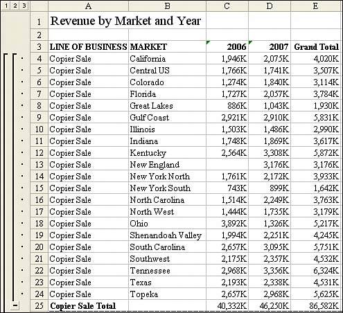
A typical report might provide a list of models with revenue by year. This report could be given to product line managers to show them which models are selling well. In this example, you want to show the models in descending order by revenue with years going across the columns. A sample report is shown in Figure 12.6.

Figure 12.6. A typical request is to take transactional data and produce a summary by model for product line managers. You can use a pivot table to get 90% of this report, and then a little formatting to finish it.

The key to producing this data quickly is to use a pivot table. Although pivot tables are incredible for summarizing data, they are quirky and their presentation is downright ugly. The final result is rarely formatted in a manner that is acceptable to line managers. There is not a good way to insert page breaks between each product in the pivot table.

To create this report, start with a pivot table that has Line of Business and Market as row fields, In Balance Date grouped by year as a column field, and Sum of Revenue as the data field. Figure 12.7 shows the default pivot table created with these settings.

Figure 12.7. Use the power of the pivot table to get the summarized data, but then use your own common sense in formatting the report.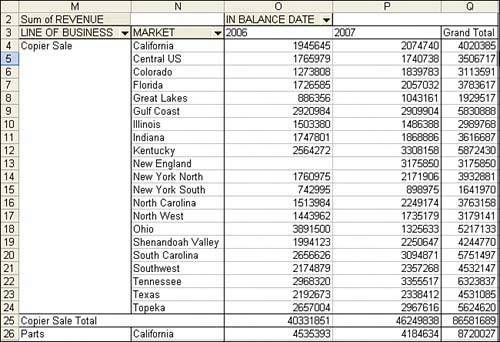

Here are just a few of the annoyances that most pivot tables present in their default state:

• The Outline view is horrible. In Figure 12.7, the value "Copier Sale" appears in the product column only once and is followed by 20 blank cells. This is the worst feature of pivot tables, and there is absolutely no way to correct it. Although humans can understand that this entire section is for product copier sales, it is radically confusing if your Copier section spills to a second or third page. Page 2 starts without any indication that the report is for copier sales. If you intend to repurpose the data, you need the Copier Sales value to be on every row.

• The report contains blank cells instead of zeroes. In Figure 12.7, customer New England had no copier sales in 2006. Excel produces a pivot table where cell O13 is blank instead of zero. This is simply bad form. Excel experts rely on being able to "ride the range," using the End and arrow keys. Blank cells ruin this ability.

• The title is boring. Most people would agree that "Sum of Revenue" is an annoying title.

• Some captions are extraneous. The words "In Balance Date" floating in cell O2 of Figure 12.7 really does not belong in a report.

• The default alphabetical sort order is rarely useful. Product line managers are going to want the top markets at the top of the list. It would be helpful to have the report sorted in descending order by revenue.

• The borders are ugly. Excel draws in a myriad of borders that really make the report look awful.

• The default number format is General. It would be better to set this up as data with commas to serve as thousands of separators, or perhaps even data in thousands or millions.

• Pivot tables offer no intelligent page break logic. If you want to be able to produce one report for each line of business manager, there is no fast method for indicating that each product should be on a new page.

• Because of the page break problem, you may find it is easier to do away with the pivot table's subtotal rows and have the Subtotal method add subtotal rows with page breaks. You need a way to turn off the pivot table subtotal rows offered for Line of Business in Figure 12.7. These show up automatically whenever you have two or more row fields. If you would happen to have four row fields, you would want to turn off the automatic subtotals for the three outermost row fields.

Even with all these problems in default pivot tables, they are still the way to go. Each complaint can be overcome, either by using special settings within the pivot table or by entering a few lines of code after the pivot table is created and then copied to a regular dataset.

Eliminate Blank Cells in the Data Area

People started complaining about the blank cells immediately when pivot tables were first introduced. Anyone using Excel 97 or later can easily replace blank cells with zeroes. In the user interface, the setting can be found in the PivotTable Options dialog box. Choose the For Empty Cells, Show option and type 0 in the box.

The equivalent operation in VBA is to set the NullString property for the pivot table to "0".

NOTE

Although the proper code is to set this value to a text zero, Excel actually puts a real zero in the empty cells.

Control the Sort Order with AutoSort

The Excel user interface offers an AutoSort option that enables you to show markets in descending order based on revenue. The equivalent code in VBA to sort the customer field by descending revenue uses the AutoSort method:

 PT.PivotFields("Line of Business").AutoSort Order:=xlDescending, _     Field:="Sum of Revenue" 

Default Number Format

To change the number format in the user interface, double-click the Sum of Revenue title, click the Number button, and set an appropriate number format.

When you have large numbers, it helps to have the thousands separator displayed. To set this up in VBA code, use the following:

 PT.PivotFields("Sum of Revenue").NumberFormat = "#,##0" 

Some companies often have customers who typically buy thousands or millions of dollars of goods. You can display numbers in thousands by using a single comma after the number format. Of course, you will want to include a "K" abbreviation to indicate that the numbers are in thousands:

 PT.PivotFields("Sum of Revenue").NumberFormat = "#,##0,K" 

Of course, local custom dictates the thousands abbreviation. If you are working for a relatively young computer company where everyone uses "K" for the thousands separator, you're in luck because Microsoft makes it easy to use the K abbreviation. However, if you work at a 100+ year-old soap company where you use "M" for thousands and "MM" for millions, you have a few more hurdles to jump. You are required to prefix the M character with a backslash to have it work:

 PT.PivotFields("Sum of Revenue").NumberFormat = "#,##0,\M" 

Alternatively, you can surround the M character with a double quote. To put a double quote inside a quoted string in VBA, you must put two sequential quotes. To set up a format in tenths of millions that uses the #,##0.0,,"MM" format, you would use this line of code:

 PT.PivotFields("Sum of Revenue").NumberFormat = "#,##0.0,,""M""" 

In case it is hard to read, the format is quote, pound, comma, pound, pound, zero, period, zero, comma, comma, quote, quote, M, quote, quote, quote. The three quotes at the end are correct. Use two quotes to simulate typing one quote in the custom number format box and a final quote to close the string in VBA.

Suppress Subtotals for Multiple Row Fields

As soon as you have more than one row field, Excel automatically adds subtotals for all but the innermost row field. However, you may want to suppress subtotals for any number of reasons. Although this may be a relatively simple task to accomplish manually, the VBA code to suppress subtotals is surprisingly complex.

You must set the Subtotals property equal to an array of 12 False values. Read the VBA help for all the gory details, but it goes something like this: The first False turns off automatic subtotals, the second False turns off the Sum subtotal, the third False turns off the Count subtotal, and so on. It is interesting that you have to turn off all 12 possible subtotals, even though Excel displays only one subtotal. This line of code suppresses the Product subtotal:

 PT.PivotFields("Line of Business").Subtotals = Array(False, False, False, False, _     False, False, False, False, False, False, False, False) 

A different technique is to turn on the first subtotal. This will automatically turn off the other 11 subtotals. You can then turn off the first subtotal to make sure that all subtotals are suppressed:

 PT.PivotFields("Line of Business").Subtotals(1) = True PT.PivotFields("Line of Business").Subtotals(1) = False 

Suppress Grand Total for Rows

Because you are going to be using VBA code to add automatic subtotals, you can get rid of the Grand Total row. If you turn off Grand Total for Rows, you delete the column called Grand Total. Thus, to get rid of the Grand Total row, you must uncheck Grand Total for Columns. This is handled in the code with the following line:

 PT.ColumnGrand = False