Setting Table Options
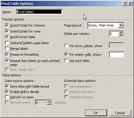
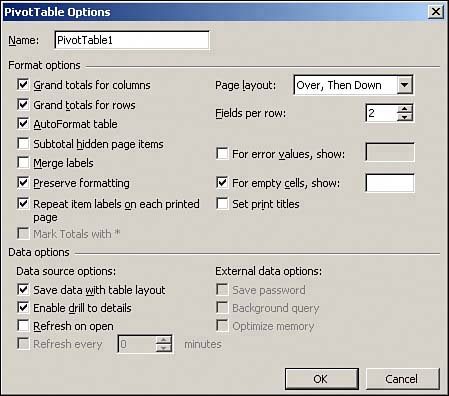
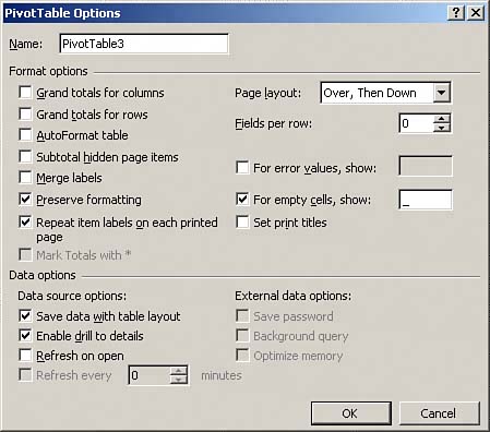
| Beyond the formatting of colors and fonts within your pivot table report, you can tweak 13 format options to modify the way your pivot data is presented and printed. These options are found in the PivotTable Options dialog box. If you regularly set these options, you can access step 3 of the PivotTable Wizard by choosing the Options button in the lower left of the dialog box. After creating a pivot table, you can activate the PivotTable Options dialog box by right-clicking inside your pivot table and selecting Table Options. Alternatively, the pivot table drop-down on the left side of the pivot table toolbar includes a Table Options selection near the bottom. The PivotTable Options dialog box is shown in Figure 4.12. The 13 options in the Format Options section are discussed next. Figure 4.12. Many important formatting options can be controlled by the PivotTable Options dialog box.
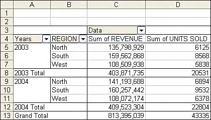
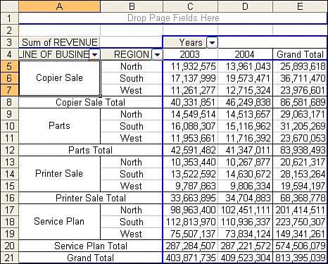
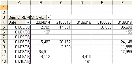
Grand Totals for ColumnsIn the table shown in Figure 4.13, the Grand Total line that adds up 2003 and 2004 does not fit in with the spirit of the report. You can remove this total by unchecking the Grand Total for Columns check box. Figure 4.13. Eliminate the Grand Total line using the PivotTable Options dialog box and unselecting Grand Totals for Columns.
Grand Totals for RowsUnselecting this option will remove the Grand Total line in the far-right column of a pivot table. AutoFormat TableChecking this option will apply the default PivotTable Classic format to your pivot table report. Removing the check from this option will allow you to preserve custom formatting you may have applied to your pivot table report. Subtotal Hidden Page ItemsChecking this option will ensure that hidden page field items will be included in the calculation of subtotals. Note that this option is not checked by default. Merged LabelsYou can select this option if you would like to merge the cells that are assigned to the label names of the data items in your row and column areas. This is relevant if you have two or more fields in either the row or column area of the pivot table. In Figure 4.14, cells A5:A7 are merged into a single cell. Cells A8:B8 are also merged into a single cell. Figure 4.14. When you have two fields in the row area, the Merge Labels option creates an interesting effect.
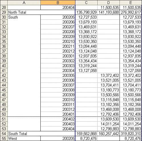
Preserve FormattingWhen this option is checked, any formatting you apply to your pivot table report is retained when you refresh or change its layout. Repeat Item Labels on Each Printed PageThis option is checked by default. When you have two row fields, Excel uses an outline view for the outer row field. In Figure 4.15, row 51 will be at the top of a new page. When you are looking at page 2, you won't really know that rows 51 through 53 apply to the South region. Figure 4.15. Due to the annoying outline view of pivot tables, you wouldn't expect to see a label of South at the top of page 2.
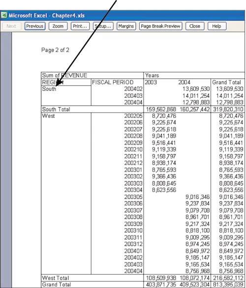
This option is one of the more amazing options in Excel. When it is checked, even though the word "South" does not appear in cell A51, Excel will ensure that the word "South" does print as if it were in cell A51. Figure 4.16 shows the page preview for page 2. Figure 4.16. The word "South" just under "Region" prints, even though that cell does not contain this word. It is one of the more amazing features of Excel.
Mark Totals with *Checking this option will mark subtotals with an asterisk if the data is based on an OLAP data source and contains values where some of the data items are hidden. This option is designed to make you aware that there are data items that are not being calculated in the subtotals. Page LayoutThis option alters the orientation of your page area layout. Typically, multiple page fields are stacked going down a column, as shown in Figure 4.17. Figure 4.17. This arrangement of page fields is due to selecting Down, Then Over from the Page Layout drop-down.
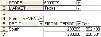
If you change the Page Layout drop-down to Over, Then Down, as shown in Figure 4.18, the page fields will stretch across a row. Figure 4.18. You can rearrange the page fields by selecting Over, Then Down from the Page Layout drop-down.
It's important to note that setting the Page Layout alone to "Over, Then Down" will merely cause your page fields to line up across the same row. To get the correct effect, this setting should be used in conjunction with the Fields per Row setting shown in Figure 4.18. Figure 4.19 shows the results of the settings in Figure 4.18. The effect is that the page fields are rearranged to line up two per row, as Fields per Row is set to 2. Figure 4.19. You can control how your page fields are displayed by using the Fields per Row setting in conjunction with the Page Layout setting.
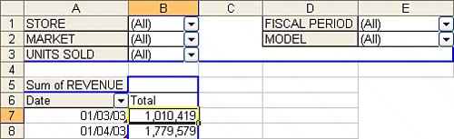
For Error Values ShowWhen you check this option, you can replace the error values in your pivot table report with any character you specify. Error values are as follows: #####, #VALUE!, #DIV/0!, #NAME?, #N/A, #REF!, #NUM!, #NULL!. For Empty Cells ShowThis is one of the more annoying features of pivot tables. In Figure 4.20, cell B7 shows that there were no sales on January 5 for store 2004014. Excel shows this by leaving the cell blank. In Chapter 3, "Customizing Fields in a Pivot Table," you learned that having blank cells instead of numeric cells can cause Excel to erroneously choose to count instead of sum data. It seems that Microsoft is breaking its own rules by leaving these cells blank instead of putting a zero in them. Figure 4.20. Excel leaves a cell blank if there are no records that show sales for a particular combination of date and store. If you would prefer to have a zero appear instead, use the For Empty Cells Show field.
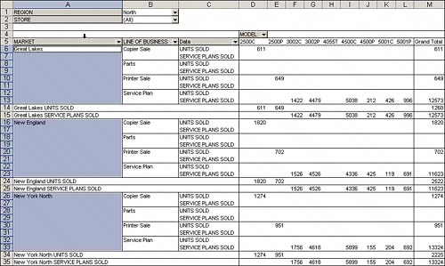
By setting the For Empty Cells Show field to a zero, you can ensure that all the fields in the data section of your pivot table have a value. Set Print TitlesIf you want to show the row and column labels in your pivot table report on each printed page of your report, check this option. CASE STUDY: Formatting a Pivot TableYou were emailed the pivot table report in Figure 4.21 and your goal is to make it easier to read and comprehend. You decide that all it needs is a few format adjustments. Here are the steps you will follow:
Figure 4.21. Your goal is to make this report easier to read.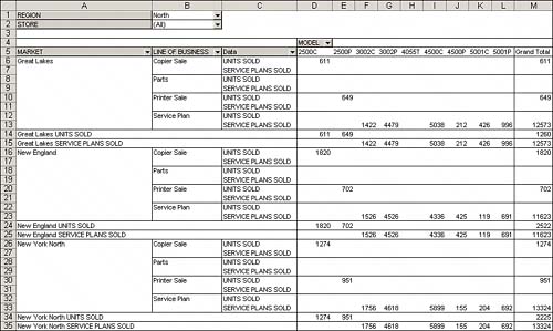
With just a few clicks, you've improved the look of your pivot table report, eliminated conspicuous empty spaces, and made your report easier to read and comprehend. The resulting pivot table is shown in Figure 4.25. Figure 4.25. The final report.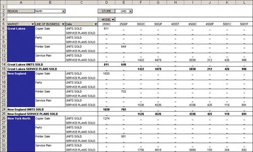 |

EAN: 2147483647
Pages: 140