Is there an easy way to fill the empty cells left by row fields?

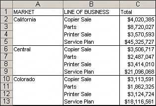
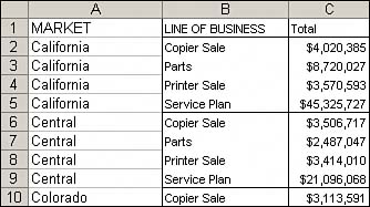
Problem

When you turn a pivot table into hard data, you are not only left with the values created by the pivot table, but you are also left with the pivot table's data structure. For example, the data shown in Figure A.9 came from a pivot table.

Figure A.9. Notice that the Market field keeps the same row field structure it had when this data was in a pivot table. It would be impractical to use this data anywhere else without filling in the empty cells left by the row field.

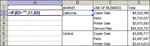
Notice that the Market field kept the same row structure it had when this data was in the row area of the pivot table. It would be unwise to use this table anywhere else without filling in the empty cells left by the row field, but how do you easily fill these empty cells?

Solution

Although the first thought that comes to your head is to copy each market and paste it into the appropriate empty cells, keep in mind that there are 20 markets. You do not want to waste your time pasting market names into empty cells.

The best solution here is to use a simple formula. This formula, shown in Figure A.10, is entered next to the first data item in the row field. The idea is to create a column next to the empty cells and fill it with a value. That value, in this case, is a market name.

Figure A.10. The formula, =IF(B2="",A1,B2), states that if the cell next to the formula is empty, use the cell above the formula. Otherwise, use the cell next to the formula.

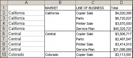
After you enter the correct formula, copy it down to the end of your dataset. As you can see in Figure A.11, this method is a lot more efficient than copying and pasting market names for 20 markets.

Figure A.11. After your formula is entered, you can copy it all the way down to the end of your dataset to fill in the gaps.

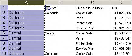
You're not done yet. After you filled in the gaps with your formula, highlight the entire column by clicking on the column letter, as shown here in Figure A.12, and then go up to the application menu and select Edit, Copy. Right-click on the column letter and select Paste Special, Values. Then click OK.

Figure A.12. Turn your formulas into hard data using Paste Special functionality.

The last step, shown in Figure A.13, is to delete the column with the empty cells and add a header to the column you just created.

Figure A.13. After a little formatting, you have the result you are looking for.