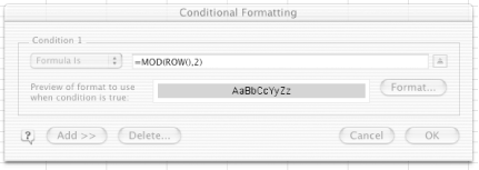
|   You've surely seen Excel spreadsheets that have alternating row colors. For instance, odd-numbered rows might be white, while even-numbered rows might be gray . Conditional formatting makes this easy . Alternating colors or shading looks professional and can make data easier to read. You can apply this formatting manually, but as you can imagine, or might have experienced , it's a rather time-consuming task that requires constant updating as you add and remove data from the table. It also requires infinite patience. Fortunately, conditional formatting can reduce the amount of patience required and enhance your professional image. We'll assume your data occupies the range A1:H100. Select this range of cells , starting with A1, thus ensuring that A1 is the active cell in the selection. Now, select Format  Conditional Formatting.... From the drop-down that currently says Cell Value Is, select Formula Is. In the Formula box, type the following formula, as shown in Figure 2-5: Conditional Formatting.... From the drop-down that currently says Cell Value Is, select Formula Is. In the Formula box, type the following formula, as shown in Figure 2-5: =MOD(ROW( ),2) Figure 2-5. Conditional Formatting dialog containing the MOD formula to specify a format to every second row in a range  Click the Format button and choose the format you want to apply to every second row. Click OK, and then click OK again. The format you specified should be applied to every second row in the range A1:H100. You also should have some patience left for the rest of the day. If you need to apply this to columns rather than rows, use this formula instead: =MOD(COLUMN( ),2) Although this method applies the formatting specified to every second row or column quickly and easily, it is not dynamic. Rows containing no data will still have the formatting applied. This looks slightly untidy and makes reading the spreadsheet a bit more difficult. Making the highlighting of every second row or column dynamic takes a little more formula tweaking. Again, select the range A1:H100, ensuring that A1 is the active cell. Select Format  Conditional Formatting..., and from the Cell Value Is pull-down menu, select Formula Is. In the Formula box, enter the following formula: Conditional Formatting..., and from the Cell Value Is pull-down menu, select Formula Is. In the Formula box, enter the following formula: =AND(MOD(ROW( ),2),COUNTA($A1:$H1))  | Note that you do not reference rows absolutely (with dollar signs), but you do reference columns this way. | |
Click the dialog's Format button and select the desired formatting, then click OK, and OK again. Any row within the range A1:H100 that does not contain data will not have conditional formatting applied. If you remove data from a specific row in your table, it too will no longer have conditional formatting applied. If you add new data anywhere within the range A1:H100, the conditional formatting will kick in. This works because when you supply a formula for conditional formatting, the formula itself must return an answer of either TRUE or FALSE . In the language of Excel formulas, 0 has a Boolean value of FALSE , while any number greater than zero has a boolean value of TRUE . When you use the formula =MOD(ROW( ),2) , it will return either a value of ( FALSE ) or a number greater than . The ROW( ) function is a volatile function that always returns the row number of the cell it resides in. You use the MOD function to return the remainder after dividing one number by another. In the case of the formula you used, you are dividing the row number by the number 2, so all even row numbers will return , while all odd row numbers will always return a number greater than . When you nest the ROW( ) function and the COUNTA function in the AND function, it means you must return TRUE (or any number greater than ) to both the MOD function and the COUNTA function for the AND function to return TRUE . COUNTA counts all nonblank cells. |