Section 3.2. T-SQL Language Enhancements

3.2. T-SQL Language Enhancements

SQL Server 2005 includes significant enhancements to the T-SQL language:

• The enhanced TOP clause supports using an expression to specify the number of rows or percent of rows returned in the result set.

• The new TABLESAMPLE clause returns a random sample of rows from the result set.

• The new OUTPUT clause returns a result set containing the rows affected by an INSERT, UPDATE, or DELETE statement.

• Common table expressions (CTEs) let you create a temporary named result set from a query, which simplifies tasks such as recursive queries.

• New SOME, ANY, and ALL operators compare the values in a column with a scalar value.

• The new PIVOT operator rotates a table, turning unique values in column rows into multiple columns in the result set, while the new UNPIVOT operator turns multiple columns in a result set into rows.

• The new APPLY operator invokes a table-valued function for each row in a result set.

• The new EXECUTE AS clause defines the user execution context of T-SQL statements.

• The new ROW_NUMBER( ), DENSE_RANK( ), and NTILE( ) ranking functions are added to the RANK function that exists in SQL Server 2000.

• New support for structured exception handling using trY...CATCH blocks.

This section details these enhancements.

3.2.1. TOP

The TOP clause limits the number of rows returned in a result set. SQL Server 2005 enhances the TOP clause to allow an expression to be used as the argument to the TOP clause instead of just a constant as was the case in SQL Server 2000. The TOP clause can be used in SELECT, INSERT, UPDATE, and DELETE statements.

The TOP clause syntax is:

     TOP (expression) [PERCENT] [ WITH TIES ] 

where:

expression

Specifies the number of rows to return or the percentage of rows in the result set to return. Parentheses are required around the expression if it is not a constant.

PERCENT

Specifies that the query should return a percent of rows from all rows processed rather than a specific number of rows.

WITH TIES

Specifies that additional rows having the same ORDER BY clause column values as the last row of the result set should be returned if they exist even though this causes the number of rows returned to be greater than specified by expression. (An example will clarify this shortly.)

The following query shows the enhanced functionality by returning the 10 products with the highest list price from the Product table in AdventureWorks. A variable is used to specify the number of rows.

     USE AdventureWorks     DECLARE @n int;     SET @n = 10;     SELECT TOP(@n)       ProductID, Name, ProductNumber, ListPrice     FROM Production.Product     ORDER BY ListPrice DESC 

Results are shown in Figure 3-2.

Figure 3-2. Results from TOP clause example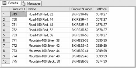

The following example shows the effect of the WITH TIES clause:

     USE AdventureWorks     SELECT TOP(6) WITH TIES       ProductID, Name, ProductNumber, ListPrice     FROM AdventureWorks.Production.Product     ORDER BY ListPrice DESC 

Results are shown in Figure 3-3.

Figure 3-3. Results from TOP WITH TIES clause example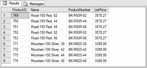

Although six rows were specified in the TOP clause, the WITH TIES clause causes the SELECT TOP statement to return an additional three rows having the same ListPrice as the value in the last row of the SELECT TOP statement without the WITH TIES clause.

3.2.2. TABLESAMPLE

The TABLESAMPLE clause returns a random, representative sample of the table expressed as either an approximate number of rows or a percentage of the total rows. Unlike the TOP clause, TABLESAMPLE returns a result set containing a sampling of rows from all rows processed by the query.

The TABLESAMPLE clause syntax is:

     TABLESAMPLE [SYSTEM] (sample_number [PERCENT | ROWS])       [REPEATABLE (repeat_seed)] 

where:

SYSTEM

An ANSI SQL keyword that specifies a database server-dependent sampling method. Although other databases support additional sampling methods that are database server-independent (e.g., DB2 supports BERNOULLI), SYSTEM is the only method supported by SQL Server 2005 and the default value if not specified.

sample_number[PERCENT | ROWS]

A numeric expression that specifies the number of rows to return or the percentage of rows in the result set to return.

REPEATABLE (repeat_seed)

The seed used to select rows to be returned in the sample. REPEATABLE indicates that the selected sample can be returned more than once. If the same seed is used, the same rows will be returned each time the query is run as long as no changes have been made to the data in the table.

The following example returns a sample result set containing the top 10 percent of rows from the Contact table:

     SELECT ContactID, Title, FirstName, MiddleName, LastName     FROM Person.Contact     TABLESAMPLE (10 PERCENT) 

The sample of rows is different every time. Adding the REPEATABLE clause as shown in the next code sample returns the same sample result set each time as long as no changes are made to the data in the table:

     SELECT ContactID, Title, FirstName, MiddleName, LastName     FROM Person.Contact     TABLESAMPLE (10 PERCENT)     REPEATABLE (5) 

The TABLESAMPLE clause cannot be used with views or in an inline table-valued function.

3.2.3. OUTPUT

The OUTPUT clause returns information about rows affected by an INSERT, UPDATE, or DELETE statement. This result set can be returned to the calling application and used for requirements such as archiving or logging.

The syntax of the OUTPUT clause is:

     <OUTPUT_CLAUSE> ::=     {         OUTPUT <dml_select_list> [ ,...n ]         INTO @table_variable     }     <dml_select_list> ::=     { <column_name> | scalar_expression }     <column_name> ::=     { DELETED | INSERTED | from_table_name } . { * | column_name } 

where:

@table_variable

A table variable into which the result set is inserted. The table variable must have the same number of columns as the OUTPUT result set, excluding identity and computed columns (which must be skipped).

<dml_select_list>

An explicit column reference (column_name) or a combination of symbols and operators that evaluates to a single value (scalar_expression).

<column_name>

An explicit column reference.

Qualify the column with the DELETED or INSERTED keyword if it references the table being modified.

from_table_name specifies the table used to provide criteria for the update or delete operation.

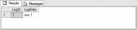
As an example, you can use the following steps to delete several rows from a table while using the OUTPUT clause to write the deleted values into a Log table variable:

1. In a new database named ProgrammingSqlServer2005, create a table called OutputTest and add three rows to it:

        USE ProgrammingSqlServer2005     CREATE TABLE OutputTest     (         ID int NOT NULL,         Description varchar(max) NOT NULL,     )     INSERT INTO OutputTest (ID, Description) VALUES (1, 'row 1')     INSERT INTO OutputTest (ID, Description) VALUES (2, 'row 2')     INSERT INTO OutputTest (ID, Description) VALUES (3, 'row 3') 

   
   

2. Execute the following query to delete the row with ID = 1 from the OutputTest table. Use the OUTPUT clause to write the deleted row to the @DeleteLog table variable.

        DECLARE @DeleteLog AS TABLE (LogID INT, LogEntry VARCHAR(MAX))     DELETE OutputTest     OUTPUT DELETED.ID, DELETED.Description INTO @DeleteLog     WHERE ID = 1     SELECT * FROM @DeleteLog 

   
   

   The last line in the query displays the log result set in the @DeleteLog table variable after the row is deleted from the OutputTest table, as shown in Figure 3-4.

   Figure 3-4. Results from OUTPUT clause example

   

When the OUTPUT clause is used for an UPDATE command, both a DELETED and INSERTED table are availablethe DELETED table contains the values before the update and the INSERTED table contains the values after the update.

3.2.4. Common Table Expressions (CTEs)

A common table expression (CTE) is a temporary named result set derived from a simple query within the scope of a SELECT, INSERT, DELETE, UPDATE, or CREATEVIEW statement. A CTE can reference itself to create a recursive CTE. A CTE is not stored and lasts only for the duration of its containing query.

The CTE syntax is:

     [WITH <common_table_expression> [ , ...n]]     <common_table_expression>::=       expression_name [(column_name [ , ...n])]       AS       (query_definition) 

where:

expression_name

Specifies the name of the CTE.

column_name

Specifies the column name in the CTE, unique within the definition. The number of column names must match the number of columns returned by the CTE query query_definition. The list of column names is optional if distinct names are returned for all columns in the CTE query.

query_definition

Specifies the SELECT statement that populates the CTE.

The following query uses a CTE to display the number of employees directly reporting to each manager in the Employee table in AdventureWorks:

     USE AdventureWorks;     WITH ManagerEmployees(ManagerID, EmployeesPerManager) AS     (       SELECT ManagerID, COUNT(*)       FROM HumanResources.Employee       GROUP BY ManagerID     )     SELECT ManagerID, EmployeesPerManager     FROM ManagerEmployees     ORDER BY ManagerID 

The query returns the results partially shown in Figure 3-5.

Figure 3-5. Results from CTE example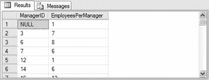

Although this example can be accomplished without a CTE, it is useful to illustrate the basic syntax of a CTE.

The WITH clause requires that the statement preceding it be terminated with a semicolon (;).

The next example uses a recursive CTE to return a list of employees and their managers:

     USE AdventureWorks;     WITH DirectReports(         ManagerID, EmployeeID, Title, FirstName, LastName, EmployeeLevel) AS     (         SELECT   e.ManagerID, e.EmployeeID, e.Title, c.FirstName, c.LastName,             0 AS EmployeeLevel         FROM HumanResources.Employee e         JOIN Person.Contact AS c ON e.ContactID = c.ContactID         WHERE ManagerID IS NULL         UNION ALL         SELECT e.ManagerID, e.EmployeeID, e.Title, c.FirstName, c.LastName,             EmployeeLevel + 1         FROM HumanResources.Employee e             INNER JOIN DirectReports d ON e.ManagerID = d.EmployeeID             JOIN Person.Contact AS c ON e.ContactID = c.ContactID     )     SELECT *     FROM DirectReports 

The query returns the results shown in Figure 3-6.

Figure 3-6. Results from recursive CTE example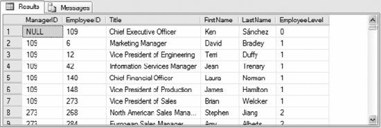

A recursive CTE must contain at least two CTE query definitionsan anchor member and a recursive member. The UNION ALL operator combines the anchor member with the recursive member.

The first SELECT statement retrieves all top-level employeesthat is, employees without a manager (ManagerID IS NULL). The second SELECT statement after the UNION ALL operator recursively retrieves the employees for each manager (employee) until all employee records have been processed.

Finally, the last SELECT statement retrieves all the records from the recursive CTE, which is named DirectReports.

You can limit the number of recursions by specifying a MAXRECURSION query hint. The following example adds this hint to the query in the previous example, limiting the result set to the first three levels of employeesthe anchor set and two recursions:

     USE AdventureWorks;     WITH DirectReports(         ManagerID, EmployeeID, Title, FirstName, LastName, EmployeeLevel) AS     (         SELECT e.ManagerID, e.EmployeeID, e.Title, c.FirstName, c.LastName,             0 AS EmployeeLevel         FROM HumanResources.Employee e         JOIN Person.Contact AS c ON e.ContactID = c.ContactID         WHERE ManagerID IS NULL         UNION ALL         SELECT e.ManagerID, e.EmployeeID, e.Title, c.FirstName, c.LastName,             EmployeeLevel + 1         FROM HumanResources.Employee e             INNER JOIN DirectReports d ON e.ManagerID = d.EmployeeID             JOIN Person.Contact AS c ON e.ContactID = c.ContactID     )     SELECT *     FROM DirectReports     OPTION (MAXRECURSION 2) 

The query results are a subset of the result set in the previous example, and are limited to an EmployeeLevel of 0, 1, or 2. The error message shown in Figure 3-7 is also displayed, indicating that the recursive query was stopped before it completed:

Figure 3-7. Message from MAXRECURSION clause in recursive CTE example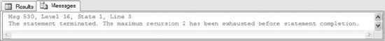

3.2.5. SOME and ANY

The SOME and ANY operators are used in a WHERE clause to compare a scalar value with a single-column result set of values. A row is returned if the scalar comparison with the single-column result set has at least one match. SOME and ANY are semantically equivalent.

The syntax of the SOME and ANY operators is:

     <scalar_expression> { = | <> | != | > | >= | !> | < | <= | !<}         {SOME | ANY} {subquery} 

where:

<scalar_expression>

A T-SQL expression.

{ = | <> | != | > | >= | !> | < | <= | !<}

A comparison operator.

<subquery>

A query that returns a single-column result set. The data type of the column must match that of the scalar expression.

The following query returns from the Person.Address table in AdventureWorks all the employee addresses that are in Canada:

     USE AdventureWorks     SELECT AddressLine1, City     FROM Person.Address     WHERE StateProvinceID = ANY       (SELECT StateProvinceID        FROM Person.StateProvince        WHERE CountryRegionCode = 'CA') 

Partial results are shown in Figure 3-8.

Figure 3-8. Results from ANY clause example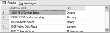

3.2.6. ALL

Use the ALL operator in a WHERE clause to compare a scalar value with a single-column result set. A row is returned if the scalar comparison to the single-column result set is true for all values in the column.

The syntax of the ALL operator is:

     <scalar_expression> { = | <> | != | > | >= | !> | < | <= | !<}         {SOME | ANY} {subquery} 

where:

<scalar_expression>

A T-SQL Server expression.

{ = | <> | != | > | >= | !> | < | <= | !<}

A comparison operator.

<subquery>

A query that returns a single column. The data type of the column must be implicitly convertible to the data type of the scalar expression.

The following query returns all the employee addresses that are not in Canada:

     USE AdventureWorks     SELECT AddressLine1, City     FROM Person.Address     WHERE StateProvinceID != ALL       (SELECT StateProvinceID        FROM Person.StateProvince        WHERE CountryRegionCode = 'CA') 

Partial results are shown in Figure 3-9.

Figure 3-9. Results from ALL clause example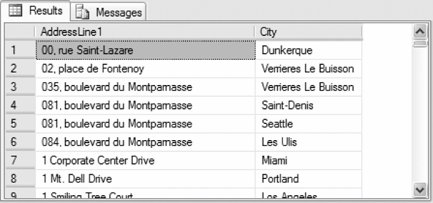

3.2.7. PIVOT and UNPIVOT

The PIVOT and UNPIVOT operators manipulate a table-valued expression into another table. These operators are essentially opposites of each otherPIVOT takes rows and puts them into columns, whereas UNPIVOT takes columns and puts them into rows.

PIVOT rotates unique values in one column into multiple columns in a result set.

The syntax of the PIVOT operator is:

     <pivoted_table> ::=         table_source PIVOT <pivot_clause> table_alias     <pivot_clause> ::=         ( aggregate_function ( value_column )             FOR pivot_column             IN ( <column_list>)         )     <column_list> ::=          column_name [, ...] 

where:

table_source

The table, view, or derived table to use in the T-SQL statement.

table_alias

An alias for table_sourcethis is required for PIVOT operators.

aggregate_function

A system- or user-defined aggregate function. COUNT(*) is not allowed.

value_column

The column containing the pivoted value.

pivot_column

The column containing the values into which the value_column aggregate values are grouped. These values are the pivot columns.

<column_list>

The pivot column names of the output table.

The following example sums the total orders by each employee in AdventureWorks for the years 2002, 2003, and 2004; pivots the total amount by year; and sorts the result set by employee ID:

     USE AdventureWorks     SELECT EmployeeID, [2002] Y2002, [2003] Y2003, [2004] Y2004     FROM       (SELECT YEAR(OrderDate) OrderYear, EmployeeID, TotalDue       FROM Purchasing.PurchaseOrderHeader) poh     PIVOT     (       SUM(TotalDue)       FOR OrderYear IN       ([2002], [2003], [2004])     ) pvt     ORDER BY EmployeeID 

Partial results are shown in Figure 3-10.

The PIVOT operator specifies the aggregate function, in this case SUM(TotalDue), and the column to pivot on, in this case OrderYear. The column list specifies that pivot columns 2002, 2003, and 2004 are displayed.

UNPIVOT does the opposite of PIVOT, rotating multiple column values into rows in a result set. The only difference is that NULL column values do not create rows in the UNPIVOT result set.

The following is the syntax of the UNPIVOT operator:

     <unpivoted_table> ::=         table_source UNPIVOT <unpivot_clause> table_alias     <unpivot_clause> ::=         ( value_column FOR pivot_column IN ( <column_list> ) )     <column_list> ::=          column_name [, ...] 

Figure 3-10. Results from PIVOT operator example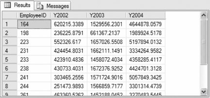

The arguments are the same as those for the PIVOT operator.

The following example unpivots the results from the previous example:

     USE AdventureWorks     SELECT EmployeeID, OrderYear, TotalDue      FROM     (       SELECT EmployeeID, [2002] Y2002, [2003] Y2003, [2004] Y2004       FROM         (SELECT YEAR(OrderDate) OrderYear, EmployeeID, TotalDue         FROM Purchasing.PurchaseOrderHeader) poh       PIVOT       (         SUM(TotalDue)         FOR OrderYear IN         ([2002], [2003], [2004])       ) pvt     ) pvtTable     UNPIVOT       (         TotalDue FOR OrderYear IN (Y2002, Y2003, Y2004)       ) unpvt     ORDER BY EmployeeID, OrderYear 

The unpivot code added to the previous example is in bold. Partial results are shown in Figure 3-11.

The UNPIVOT operator clause specifies the value to unpivot, in this case TotalDue, and the column to unpivot on, in this case OrderYear. As expected, the results match the pivoted column values in the previous example.

Figure 3-11. Results from UNPIVOT operator example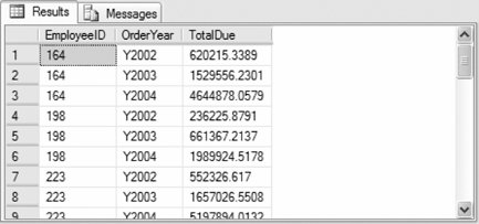

3.2.8. APPLY

The APPLY operator invokes a table-valued function for each row returned by an outer table expression of a query. The table-valued function is evaluated for each row in the result set and can take its parameters from the row.

There are two forms of the APPLY operatorCROSS and OUTER. CROSSAPPLY returns only the rows from the outer table where the table-value function returns a result set. OUTERAPPLY returns all rows, returning NULL values for rows where the table-valued function does not return a result set.

The syntax for the APPLY operator is:

     {CROSS | OUTER} APPLY {table_value_function} 

where:

table_value_function

Specifies the name of a table-valued function

Let's walk through an example using the APPLY operator to return sales order detail records from AdventureWorks for a sales order header where the order quantity is at least the minimum quantity specified. You can do this using a traditional JOIN. However, this example uses the APPLY operator and the following table-valued function:

     USE AdventureWorks     GO     CREATE FUNCTION tvfnGetOrderDetails       (@salesOrderID [int], @minOrderQuantity [smallint])     RETURNS TABLE     AS     RETURN     (         SELECT *         FROM Sales.SalesOrderDetail         WHERE         SalesOrderID = @salesOrderID AND         OrderQty > @minOrderQuantity     ) 

You must add a GO command after the USE statement, because the CREATEFUNCTION must be the first statement in a query batch.

The following CROSSAPPLY query returns the SalesOrderID and OrderDate from the SalesOrderHeader together with the ProductID for lines where more than one item was ordered:

     USE AdventureWorks     SELECT soh.SalesOrderID, soh.OrderDate,       sod.ProductID, sod.OrderQty     FROM Sales.SalesOrderHeader soh     CROSS APPLY       tvfnGetOrderDetails(soh.SalesOrderID, 1) sod     ORDER BY soh.SalesOrderID, sod.ProductID 

Partial results are shown in Figure 3-12.

Figure 3-12. Results from CROSS APPLY operator example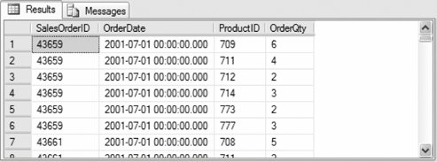

The result set contains only sales order detail rows where more than one item is ordered. Sales order 43660 does not have any detail lines with more than one item ordered, so the CROSS APPLY operator does not return a row for that order.

Change the query to use the OUTER APPLY operator:

     USE AdventureWorks     SELECT soh.SalesOrderID, soh.OrderDate, sod.ProductID, sod.OrderQty     FROM Sales.SalesOrderHeader soh     OUTER APPLY tvfnGetOrderDetails(soh.SalesOrderID, 1) sod     ORDER BY soh.SalesOrderID 

The results are similar to those returned using the CROSS APPLY operator, except that order 43660 is now included in the result set, with NULL values for the two columns from the table-value function. Partial results are shown in Figure 3-13.

Figure 3-13. Results from OUTER APPLY operator example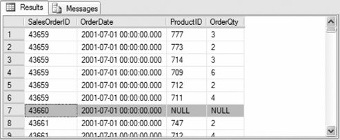

3.2.9. EXECUTE AS

SQL Server 2005 lets you define the execution context of the following user-defined modules: functions, stored procedures, queues, and triggers (both DML and DDL). You do this by specifying the EXECUTEAS clause in the CREATE and ALTER statements for the module. Specifying the execution context lets you control the user account that SQL Server uses to validate permissions on objects referenced by the modules.

The syntax of the EXECUTEAS clause is given next for each of the categories items for which you can define the execution context:

Functions, stored procedures, and DML triggers:

     EXECUTE AS { CALLER | SELF | OWNER | 'user_name' } 

DDL triggers with database scope:

     EXECUTE AS { CALLER | SELF | 'user_name' } 

DDL triggers with server scope:

     EXECUTE AS { CALLER | SELF | 'login_name' } 

Queues:

     EXECUTE AS { SELF | OWNER | 'user_name' } 

where:

CALLER

Statements inside the module execute in the context of the caller of the module. CALLER is the default for all modules except for queues for which the CALLER context is not valid.

SELF

Statements inside the module execute in the context of the person creating or altering the module. SELF is the default for queues.

OWNER

Statements inside the module execute in the context of the current owner of the module.

'user_name'

Statements inside the module execute in the context of the user specified in 'user_name'.

'login_name'

Statements inside the module execute in the context of the SQL Server login specified in 'login_name'.

For more information about specifying execution context, see Microsoft SQL Server 2005 Books Online.

3.2.10. New Ranking Functions

SQL Server 2005 introduces three new ranking functions : ROW_NUMBER( ), DENSE_RANK( ), and NTILE( ). This is in addition to the RANK( ) function available in SQL Server 2000.

3.2.10.1. ROW_NUMBER( )

The ROW_NUMBER( ) function returns the number of a row within a result set starting with 1 for the first row. The ROW_NUMBER( ) function does not execute until after a WHERE clause is used to select the subset of data.

The ROW_NUMBER( ) function syntax is:

     ROW_NUMBER(  ) OVER ([<partition_by_clause>] <order_by_clause>) 

where:

<partition_by_clause>

Divides the result set into groups to which the ROW_NUMBER( ) function is applied. The function is applied to each partition separately; computation restarts for each partition.

<order_by_clause>

Specifies the order in which the sequential ROW_NUMBER( ) values are assigned.

The following example returns the row number for each contact in AdventureWorks based on the LastName and FirstName:

     USE AdventureWorks     SELECT ROW_NUMBER(  ) OVER(ORDER BY LastName, FirstName),       ContactID, FirstName, LastName     FROM Person.Contact 

Partial results are shown in Figure 3-14.

Figure 3-14. Results from ROW_NUMBER( ) function example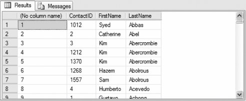

The following example uses the PARTITION BY clause to rank the same result set within each manager:

     USE AdventureWorks     SELECT ManagerID, ROW_NUMBER(  )       OVER(PARTITION BY ManagerID ORDER BY LastName, FirstName),       e.ContactID, FirstName, LastName     FROM HumanResources.Employee e     LEFT JOIN Person.Contact c       ON e.ContactID = c.ContactID 

Partial results are shown in Figure 3-15.

Figure 3-15. Results from PARTITION BY clause example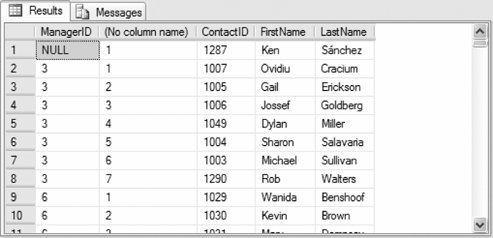

The row numbers now restart at 1 for each manager. The employees are sorted by last name and then first name for each manager group.

3.2.10.2. DENSE_RANK( )

The DENSE_RANK( ) function returns the rank of rows in a result set without gaps in the ranking . This is similar to the RANK( ) function except that in cases where more than one row receives the same ranking, the next rank value is the rank of the tied group plus 1 rather than the next row number.

The DENSE_RANK( ) function syntax is:

     DENSE_RANK(  ) OVER ([<partition_by_clause>] <order_by_clause>) 

where:

<partition_by_clause>

Divides the result set into groups to which the ROW_NUMBER( ) function is applied. The function is applied to each partition separately; computation restarts for each partition.

<order_by_clause>

Specifies the order in which the sequential DENSE_RANK( ) values are assigned.

The following example shows the difference between DENSE_RANK( ) and the RANK( ) function by ranking contacts in AdventureWorks based on last name:

     USE AdventureWorks     SELECT       DENSE_RANK(  ) OVER(ORDER BY LastName) DenseRank,       RANK(  ) OVER(ORDER BY LastName) Rank,       ContactID, FirstName, LastName     FROM Person.Contact 

Partial results are shown in Figure 3-16.

Figure 3-16. Results from DENSE_RANK( ) function example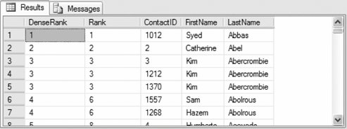

3.2.10.3. NTILE( )

The NTILE( ) function returns the group in which a row belongs within an ordered distribution of groups. Group numbering starts with 1.

The NTILE( ) function syntax is:

     NTILE(n) OVER ([<partition_by_clause>] <order_by_clause>) 

where:

n Specifies the number of groups that each partition should be divided into.

<partition_by_clause>

Divides the result set into groups to which the NTILE( ) function is applied. The function is applied to each partition separately; computation restarts for each partition.

<order_by_clause>

Specifies the column used to define the groups to which the NTILE( ) function is applied.

The following query distributes product list prices from AdventureWorks into four groups:

     USE AdventureWorks     SELECT NTILE(4) OVER (ORDER BY ListPrice) GroupID,       ProductID, Name, ListPrice     FROM Production.Product     WHERE ListPrice > 0     ORDER BY Name 

Partial results are shown in Figure 3-17.

Figure 3-17. Results from NTILE( ) function example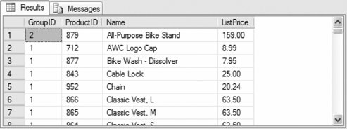

If the number of rows is not evenly divisible by the number of groups, the size of the groups will differ by one.

3.2.11. Error Handling

SQL Server 2005 introduces structured exception handling similar to that found in C#. A group of T-SQL statements can be enclosed in a trY block. If an error occurs within the trY block, control is passed to a CATCH block containing T-SQL statements that handle the exception. Otherwise execution continues with the first statement following the CATCH block. If a CATCH block executes, control transfers to the first statement following the CATCH block once the CATCH block code completes.

A TRY...CATCH block does not trap warningsmessages with severity of 10 or loweror errors with a severity level greater than 20errors that typically terminate the Database Engine task.

trY...CATCH blocks are subject to the following rules:

• A trY block must be followed immediately by its associated CATCH block.

• Each trY...CATCH block must be contained in a single batch, stored procedure, trigger, or function. A trY block cannot span multiple batchesfor example, more than one BEGIN...ELSE block or IF...ELSE block.

• trY...CATCH blocks can be nested.

• You can use a GOTO statement to transfer control within a trY or CATCH block or to exit a TRY or CATCH block. You cannot use a GOTO statement to enter a TRY or CATCH block.

The trY...CATCH syntax is:

     BEGIN TRY     { sql_statement | sql_statement_block }     END TRY     BEGIN CATCH     { sql_statement | sql_statement_block }     END CATCH 

where:

sql_statement

A T-SQL statement

sql_statement_block

A group of T-SQL statements enclosed in a BEGIN...END block

For example, the Employee table in AdventureWorks has a check constraint that the Gender column can contain only M or F. The following statement updates the Gender for the employee with EmployeeID = 1 with the invalid value X:

     USE AdventureWorks     BEGIN TRY       UPDATE HumanResources.Employee       SET Gender = 'X'       WHERE EmployeeID = 1;     END TRY     BEGIN CATCH       SELECT ERROR_NUMBER(  ) ErrorNumber,       ERROR_STATE(  ) ErrorState,       ERROR_SEVERITY(  ) ErrorSeverity,       ERROR_MESSAGE(  ) ErrorMessage;     END CATCH 

Executing this code returns a result set containing error information:

Column	Value
ErrorNumber	547
ErrorState	0
ErrorSeverity	16
ErrorMessage	UPDATE statement conflicted with CHECK constraint 'CK_Employee_Gender'. The conflict occurred in database 'AdventureWorks', table 'Employee', column 'Gender'.

As shown in the example, you can use the following functions to return information about the error caught by a CATCH block:

ERROR_MESSAGE( )

Diagnostic information about the error. These messages often contain substitution variables that allow specific information, such as the database object that caused the error, to be included in the message.

ERROR_NUMBER( )

The unique error number of the error. The ERROR_NUMBER( ) function returns the last error number every time it is called. This is different from @@ERROR, which works only if it immediately follows the error or is the first statement in the CATCH block.

ERROR_SEVERITY( )

The severity level of the error. Error severities range from 0 to 24. Error levels 0 to 9 are warnings or informational.

ERROR_STATE( )

The state of the error. A state code uniquely identifies specific conditions that cause errors with the same error number.