Using Functions to Analyze Finances

Although Excel includes too many functions to discuss exhaustively in this book, we thought you might enjoy seeing a few more examples of functions and formulas to prompt your own exploration. We've decided to highlight three of Excel's most useful financial functions: PMT, FV, and RATE. Using these functions, you can precisely calculate loan payments, the future value of an investment, or the rate of return produced by an investment.

Using PMT to Determine Loan Payments

The PMT function returns the periodic payment required to amortize a loan over a set number of periods. In plain English, this means that you can estimate what your car payments will be if you take out an auto loan or what your mortgage payments will be if you buy a house. Try using the PMT function now to determine what the monthly payments will be for a $10,000 auto loan at 9 percent interest over a 3-year period.

To use the PMT function, follow these steps:

1. Click the worksheet cell in which you want to display the monthly payment.
2. Choose Function from the Insert menu, or click the Paste Function button on the Standard toolbar. The Paste Function dialog box appears.
3. Click the Financial category, and then double-click PMT in the Function Name list box. The arguments dialog box appears. It contains a description of the PMT function and five text boxes ready to accept the function's arguments. You'll enter numeric values for rate (the interest rate), nper (the number of payments), and pv (the present value, or loan principal).
4. Type 9%/12 and press Tab, type 36 and press Tab, and type 10000. The dialog box should look like this:



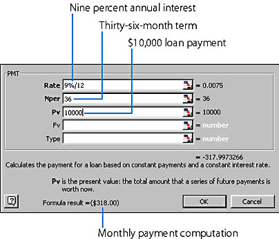
The result of the calculation ($318.00) is displayed near the bottom of the dialog box.

TIP

---

To calculate monthly payments, be sure to type the annual interest using a percent sign and divide it by 12 to create a monthly interest rate. Likewise, be sure to specify the number of payments in months (36), not years (3).

5. Click OK to complete the function and display the result. Your monthly loan payment, less any applicable loan fees, appears in the cell you highlighted. The result, formatted as currency, is ($318.00). The amount appears in red and between parentheses because it represents money that you must pay out.

Using FV to Compute Future Value

Although monthly loan payments are often a fact of life, Excel can help you with more than just debt planning. If you enjoy squirreling away money for the future, you can use the FV (future value) function to determine the future value of an investment. Financial planners use this tool when they help you to determine the future value of an annuity, IRA, or SEP account. The following example shows you how to compute the future value of an IRA in which you deposit $2,000 per year for 30 years at a 10 percent annual interest rate— a possible scenario if you invested $2,000 per year between the ages of 35 and 65.

To use the FV function to calculate the value of your investment at retirement, follow these steps:

1. Click the worksheet cell in which you want to display the investment total.
2. Open the Paste Function dialog box.
3. Click the Financial category, and then double-click FV in the Function Name list box.

A dialog box appears that contains a description of the FV function and five text boxes for the function's arguments. (The arguments are related to those of the PMT function, but now a Pmt field is added so that you can enter the amount you're contributing each period.)

4. Type 10% in the Rate text box and press Tab, type 30 in the Nper text box and press Tab, type -2000 in the Pmt text box and press Tab twice, and then type 1 in the Type text box.

Note that Rate and Nper must be based on the same units of time. In the previous example months were the basis; here, years are the basis for the calculation. Your dialog box should look like the following:



5. Click OK to display the result.

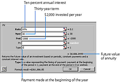
In our example, the 30-year IRA has a future value of $361,886.85. Not bad for a total investment of $60,000.

NOTE

---

By placing a 1 in the Type text box, you direct Excel to start calculating each year's interest at the beginning of the year— a sensible move if you place one lump sum in your IRA at the same time each year. If you omit this argument, Excel will calculate each year's interest at the end of the year, and the total future value will be smaller— about $33,000 less in this example.

Using RATE to Evaluate Rate of Return

You'll often want to evaluate how a current investment is doing or how a new business proposition looks. For example, suppose that a contractor friend suggests you loan him $10,000 for a laundromat/brew pub project, and agrees to pay you $3,200 per year for four years as a minimum return on your investment. So what's the projected rate of return for this investment opportunity? You can figure it out quickly using the RATE function, which allows you to determine the rate of return for any investment that generates a series of periodic payments or a single lump-sum payment.

To use the RATE function to determine the rate of return for an investment, follow these steps:

1. Click the worksheet cell in which you want to display the rate of return.
2. Open the Paste Function dialog box.
3. Click the Financial category, scroll down in the Function Name list box, and then double-click RATE.

A dialog box appears that contains a description of the RATE function and six text boxes for the function's arguments. (Scroll down to see the sixth text box, Guess.) The arguments are similar to the ones you have used in previous financial functions, but they appear in a slightly different order.

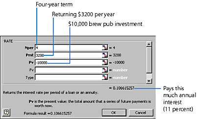
4. Type 4 in the Nper text box and press Tab, type 3200 in the Pmt text box and press Tab, and type -10000 in the Pv text box. Your dialog box should look like this:



5. Click OK to display the result. In this example, your investment of $10,000 today will return 11 percent annually if your friend regularly pays you $3,200 per year for the next four years. With this information in hand, you can decide whether the projected rate of return is enough for you, or whether you'd rather try something less risky— or renegotiate the deal.

In short, Excel functions can't guarantee your financial success, but when used correctly, they can help you make decisions based on the best data available.

Using Function Error Values

The Paste Function dialog box makes entering functions relatively straightforward. If you do make a mistake when typing a function, you might receive a code called an error value in one or more cells. Error values begin with a pound (#) symbol and usually end with an exclamation point. For example, the error value #NUM! means that the function arguments you supplied aren't sufficient to calculate the function— one of the arguments might be too big or too small. If you see an error value in a cell, simply click the cell and fix your mistake on the formula bar, or delete the formula and enter it again. (If you're building a function, use the function's online Help to double-check your arguments.) Table 20-3 shows the most common Excel error values and their meanings.

Table 20-3. Common Error Values in Excel Formulas

Error Value	Description
#DIV/0!	You're dividing by zero in this formula. Verify that no cell references refer to blank cells.
#NA	You might have omitted a function argument. No value is available.
#NAME?	You're using a range name in this formula that hasn't been defined in the workbook. (See the next section, "Using Range Names in Functions")
#NULL!	You attempted to use the intersection of two areas that don't intersect (are not contiguous). You might have an extra space character in one of your range arguments.
#NUM!	Your function arguments might be out of range or otherwise invalid, or an iterative function you're using might not have computed long enough to reach a solution. (Entering a rough answer in the Guess argument might reduce the number of iterations Excel needs.)
#REF!	Your formula includes range references that have been deleted.
#VALUE!	Your formula is using a text entry as an argument.
######	Your calculation results were too wide to fit in the cell. Increase the column width.