Using Built-In Functions
To accomplish more sophisticated numerical and text processing operations in your worksheets, Excel allows you to add built-in calculations called functions to your formulas. A function is a predefined equation that operates on one or more values and returns a single value. Excel includes a collection of over 200 functions in several useful categories, as shown in Table 20-2. For example, you can use the PMT (payment) function from the Financial category to calculate the periodic payment for a loan based on the interest rate charged, the number of payments desired, and the principal amount.
SEE ALSO
For more information on the PMT function, see "Using PMT to Determine Loan Payments"
Each function must be entered with a particular syntax, or structure, so that Excel can process the results correctly. For example, the PMT function has a function syntax that looks like this:
PMT(rate,nper,pv,fv,type)
Table 20-2. Categories of Excel Functions
| Category | Used For |
|---|---|
| Financial | Loan payments, appreciation, and depreciation |
| Date & Time | Calculations involving dates and times |
| Math & Trig | Mathematical and trigonometric calculations like those found on a scientific calculator |
| Statistical | Average, sum, variance, and standard-deviation calculations |
| Lookup & Reference | Calculations involving tables of data |
| Database | Working with lists and external databases |
| Text | Comparing, converting, and reformatting text in cells |
| Logical | Calculations that produce the result TRUE or FALSE |
| Information | Determining whether an error has occurred in a calculation |
The abbreviated words shown between the parentheses are called arguments. In this function, rate is the interest rate, nper is the number of payments you'll make, and pv is the principal amount. To use this function correctly, you must specify a value for each required argument, and you must separate each argument with a comma. The arguments shown in bold are required, and the others are optional. (In the online Help, the optional arguments are also in bold.) For example, to use the PMT function to calculate the loan payment on a $1,000 loan at 19 percent annual interest over 36 months, you could type the following formula:
=PMT(19%/12,36,1000)
When Excel evaluates this function, it places the answer ($36.66) in the cell containing the function. (The answer is negative, indicated by the parentheses, because it is money you must pay out.) Note that the first argument (the interest rate) was divided by 12 in this example to create a monthly rate for the formula. This demonstrates an important point— you can use other calculations, including other functions, as the arguments for a function. Although it takes a little time to master how these arguments are structured, you'll find that functions produce results that can otherwise take hours to calculate by hand.
The Versatile SUM Function
Perhaps the most useful function in Excel's collection is SUM, which totals the range of cells you select. Because SUM is used so often, the AutoSum button appears on the Standard toolbar to make adding numbers faster. In the following example, we'll use the AutoSum button to sum the Subtotal column in the order-form worksheet.

To total a column of numbers using the SUM function, follow these steps:
- Click the cell in which you want to place the SUM function. (If you're totaling a column of numbers, select the cell directly below the last number in the column.)
- Click the AutoSum button.
- If Excel selected the range you want to total, press Enter to complete the function and compute the sum. If Excel didn't guess the range correctly, select a new range now by dragging the mouse over the range and pressing Enter. (You can specify any block of cells in any open workbook to be an argument to the SUM function.) To cancel the AutoSum command, press the Escape key.
Excel places the SUM function on the formula bar, and (if possible) automatically selects a range of neighboring cells as an argument for the function. If you selected a cell directly below a column of numbers, your screen will look similar to the one in Figure 20-2.
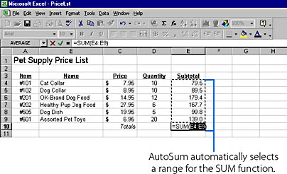
Figure 20-2. The AutoSum button inserts the SUM function and automatically suggests the cells to use for the argument.
TIP
Use SUM to Add Nonadjacent RangesYou can use the SUM function to add multiple noncontiguous ranges by separating the cell ranges with commas. For example, =SUM(A3:A8,B3:B8) adds six cells in column A to six cells in column B and displays the total. You might find it easier to use the mouse and select cells by clicking each cell or range of cells while pressing the Ctrl key.
The Insert Function command
With so many functions to choose from, it might seem daunting to experiment with unfamiliar features on your own. Excel makes it easier by providing a special command named Function on the Insert menu, to help you learn about functions and enter them into formulas. The Paste Function dialog box, shown in Figure 20-3, lets you browse through the nine function categories and pick just the calculation you want.
You can also use Office Assistant to help you learn how each function works and what arguments it requires. (More than 200 functions are carefully documented in the online Help.) When you double-click a function in the Function Name list box, Excel displays a second dialog box prompting you for the required arguments. Give it a try now with a useful statistical function called AVERAGE.
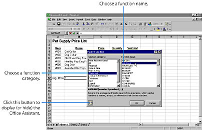
Figure 20-3. The Paste Function dialog box lists function names by category.
To use AVERAGE to calculate the average of a list of numbers, follow these steps:
- Click the cell in which you want to place the results of the AVERAGE function. (In the pet-shop example, this is B12. The label Avg. Price has been added in A12.)
- From the Insert menu, choose Function. The Paste Function dialog box appears, as shown in Figure 20-3. The nine functional categories appear in the Function Category list box along with the choice for All functions and those Most Recently Used, and the functions in each category are listed alphabetically in the Function Name list box.
- Click the Statistical category. The mathematical functions in the Statistical category appear in the Function Name list box.
- Click the AVERAGE function, and then click OK. A second dialog box appears, asking you for the arguments in the function. In the AVERAGE function, you can specify either individual values to compute the average or a cell range. This time, you'll specify a cell range.
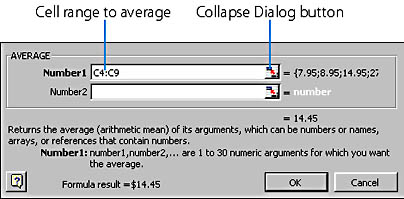
- Click the Collapse Dialog button (small red arrow at the right edge of the Number1 text box shown below), and the dialog box will shrink to show only the text box you're about to fill.
- Select the cells you want to average. In our example, we selected the numbers in the Price column (cells C4 through C9) to determine the average price of pet supplies in the store.
- Release the mouse button, and press Enter. The dialog box returns to its normal size, and the cell range you selected appears in the dialog box and in the AVERAGE function on the formula bar. Our dialog box looks like this:
- Click OK to complete the formula and calculate the result. The average, $14.45, appears in the cell containing the AVERAGE formula.
TIP
You can save time opening the Paste Function dialog box by clicking the Paste Function button on the Standard toolbar.

TIP
You can include one function as an argument in another function if the result is compatible. For example, the formula =SUM(5,SQRT(9)) adds together the number 5 and the square root of 9, and then displays the result (8).
EAN: 2147483647
Pages: 228
- Chapter I e-Search: A Conceptual Framework of Online Consumer Behavior
- Chapter IV How Consumers Think About Interactive Aspects of Web Advertising
- Chapter VIII Personalization Systems and Their Deployment as Web Site Interface Design Decisions
- Chapter IX Extrinsic Plus Intrinsic Human Factors Influencing the Web Usage
- Chapter XVIII Web Systems Design, Litigation, and Online Consumer Behavior