Building a Formula
Figure 20-1 shows two basic Excel formulas. The first calculates a value by multiplying two numbers, and the second calculates a sum by adding three cell references. These formulas have several characteristics in common.
- Each begins with an equal sign (=). The equal sign tells Excel that the following characters are part of a formula that should be calculated and that the result should be displayed in a cell. (If you omit the equal sign, Excel treats the formula as plain text and doesn't compute the result.)
- Each formula uses one or more arithmetic operators. An arithmetic operator is not required when a function is used in a formula, but in all other cases, operators are necessary to tell Excel what to do with the values in an equation. If your formula contains more than one arithmetic operator, you can include parentheses to clarify how the formula is evaluated.
- Each formula includes two or more values that are being combined by using arithmetic operators. When you use Excel formulas, you can combine numbers, cell references, and other values.
The examples in this chapter feature an order-form worksheet that catalogs the merchandise sold in a small pet shop. It's the type of worksheet that pet-shop employees might use to take orders over the phone or that customers might use to purchase mail-order items. As you work through this chapter, you'll see how to use Excel formulas and functions to add information to the order-form worksheet. You can create the worksheet and follow the examples exactly if you want to, or you can customize the worksheet for your own purposes.
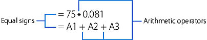
Figure 20-1. The anatomy of two simple Excel formulas.
Multiplying Numbers
Formulas that multiply the numbers in two cells are the most basic and the easiest to enter. The following example shows you how to multiply a price cell and a quantity cell to create a subtotal.
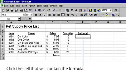
- Create a product order form, price list, or another worksheet containing well-organized Price, Quantity, and Subtotal columns. The order-form worksheet we'll use looks like this:
- In the Subtotal column, click the cell that will contain the multiplication formula (E4 in our example).
- Type the equal sign (=) to begin the formula.
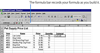
- In the Price column, click the cell containing the first number to be multiplied (C4 in this example). A dotted-line marquee appears around the highlighted cell, and the cell reference appears in the formula bar.
- Type an asterisk (*) to add the multiplication operator to the formula.
- In the Quantity column, click the cell containing the second number to be multiplied (D4 in this example). The complete formula now appears in the highlighted cell and on the formula bar. Your worksheet should look similar to the one shown below.
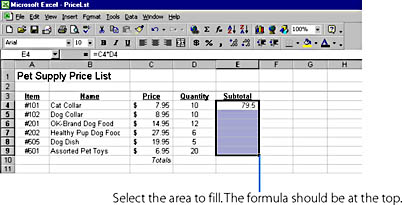
- Press Enter to end the formula. Excel calculates the result (79.5 in this example), and displays it in the cell containing the formula. Later you'll add currency formatting to the cell.
ON THE WEB
The PriceLst example is on the Running Office 2000 Reader's Corner page. For information about connecting to this Web site, read the Introduction.
An equal sign appears on the formula bar and in the highlighted cell. From this point on, any numbers, cell references, arithmetic operators, or functions that you type will be included in the formula.
SEE ALSO
To learn more about entering simple formulas, referencing cells, and using the formula bar, see "Entering Formulas"
Replicating a Formula
Excel makes it easy to copy, or replicate, a formula into neighboring cells, using the Fill submenu of the Edit menu. The slick thing about the Fill submenu is that its commands automatically adjust the cell references in your formula to match the rows and columns you're copying to. For example, if you replicate a formula down a column with the Down command, Excel adjusts the row numbers so that the formula includes new references in each cell. (Excel automatically adjusts cell references when you delete cells, too.) The following example shows you how to use the replication feature in the order-form worksheet.
SEE ALSO
For more information about the commands on the Fill submenu, see "Using the Fill Commands"
To replicate a formula, follow these steps:
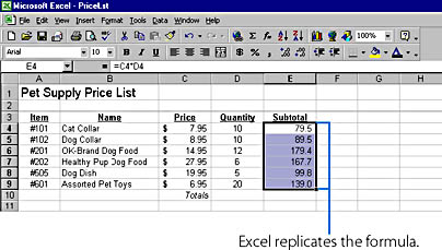
- Highlight the cell that has the formula and the empty cells you want to fill as one selection. (The Fill command replicates formulas in only one direction; commands on the Fill submenu copy to neighboring, or contiguous, cells only, so be sure that the formula cell is at the top, bottom, left, or right end of the empty cell range.) Our worksheet looks like this:
- Choose Fill from the Edit menu, and then choose Down from the submenu if your formula is at the top of the selected range, or choose Right, Left, or Up as appropriate. Your formula is replicated within the selected cells, as shown here:
- Select column E in the worksheet, and click the Currency Style button on the Formatting toolbar. The contents of the Subtotal column now appear in currency format.
SEE ALSO
To control how Excel calculates formulas, see "Controlling Calculations"
TIP
You can also replicate a formula by using the AutoFill mouse technique. Simply select the cell you want to replicate, click the tiny box in the lower right corner of the cell, and drag it over the cells you want to fill.
Using Arithmetic Operators
As you learned in the previous example, Excel lets you build your formulas by using one or more arithmetic operators to combine numbers and cell references in an equation. Table 20-1 shows a complete list of the arithmetic operators you can use in a formula. When you enter more than one arithmetic operator, Excel follows standard algebraic rules to determine which calculations to accomplish first in the formula. These rules— called Excel's order of evaluation— dictate that exponential calculations are performed first, multiplication and division calculations second, and addition and subtraction last. If more than one calculation exists in the same category, Excel evaluates them from left to right. For example, when evaluating the formula =6-5+3*4, Excel computes the answer using these steps:
=6-5+3*4
=6-5+12
=1+12
=13
Table 20-1. Excel's Arithmetic Operators, in Order of Evaluation
| Operator | Description | Example | Result |
|---|---|---|---|
| ( ) | Parentheses | (3+6)*3 | 27 |
| ^ | Exponential | 10^2 | 100 |
| * | Multiplication | 7*5 | 35 |
| / or ÷ | Division | 15÷3 | 5 |
| + | Addition | 5+5 | 10 |
| - | Subtraction | 12-8 | 4 |
Parentheses and Order of Evalutation
To change Excel's order of evaluation, you can include one or more pairs of parentheses in a formula. This lets you control how Excel uses operators in a formula, and can also make your equation easier to read and revise later. For example, consider how parentheses create a difference in evaluation between these two formulas:
=10+2*0.25
=(10+2)*0.25
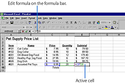
Editing FormulasExcel allows you to edit formulas in the same way that you edit any other cell entry. Simply double-click the cell, locate the mistake using the arrow keys, make your correction, and press Enter. You can also insert new cell references while editing a formula by positioning the mouse pointer on the formula bar and highlighting new cells with the mouse. This handy feature lets you specify replacement cells in your formula if you selected the wrong cells the first time.
The following example shows what a formula in cell E9 looks like when you edit it in a cell. Note that Excel places color outlines around the other cells involved in the formula to make it easy to see their relationships. If you prefer, you can also highlight a cell and click the formula bar to edit the cell s contents there. (To cancel an edit, press Escape.)
The first formula produces a result of 10.5, while the second formula produces a result of 3. By modifying Excel's order of evaluation in the second formula, you create an entirely different answer.
Parentheses can also make a formula easier to read, and you can add any number of parentheses as long as you use them in matching pairs. For example, though the following formulas both produce the answer 15, the first formula is a bit easier to decipher.
=((5*4)/2)+(10/2)
=5*4/2+10/2
NOTE
If you specify an uneven number of parentheses in a formula, or a pair of parentheses that don't match, Excel displays a message that it found an error in the formula and proposes a correction. Click Yes to accept Excel's proposed correction, or click No so you can correct the mistake on the formula bar or in the cell directly.
EAN: 2147483647
Pages: 228