Graphs

Unlike charts, which plot data interactively, graphs plot pre-generated arrays of data all at once; they do not have the ability to append new values to previously generated data. LabVIEW provides several types of graph for greater flexibility: waveform graphs, XY graphs, intensity graphs, 3D graphs, digital waveform graphs, and some specialized graphs (Smith plots, Polar charts, Min-Max, and distribution plots). We'll talk about waveform and XY graphs now and cover intensity and 3D graphs later, in the "3D Graphs" section of this chapter. Waveform graphs and XY graphs look identical on the front panel of your VI but have very different functionality.

An example of a graph with several graph options enabled is shown in Figure 8.13.

Figure 8.13. A Waveform Graph with several graph options enabled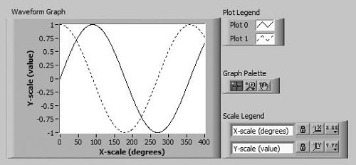

You can obtain both types of graph indicator from the Modern>>Graph subpalette of the Controls palette. The waveform graph plots only single-valued functions (only one Y value for every X) with uniformly spaced points, such as acquired time-sampled, amplitude-varying waveforms. The waveform graph is ideal for plotting arrays of data in which the points are evenly distributed.

The XY graph is a general-purpose, Cartesian graph, ideal for plotting data with varying timebases or data with several Y values for every X value, such as circular shapes. The two types of graph look the same but take different types of input, so you must be careful not to confuse them.

Single-Plot Waveform Graphs

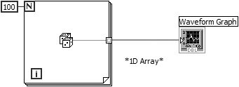
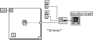
For basic single-plot graphs, you can wire an array of Y values directly to a waveform graph terminal, as shown in Figure 8.14. This method assumes the initial X value is zero, and the delta X value (i.e., the increment between X values) is one. Notice that the graph terminal in the block diagram shown in Figure 8.14 appears as an array indicator (if you deselect View as Icon from its pop-up menu).

Figure 8.14. Passing a 1D array to a Waveform Graph to display a single plot with multiple points

Recall from Chapter 7, "LabVIEW's Composite Data: Arrays and Clusters," that an auto-indexing output tunnel (which is enabled by default for tunnels on For Loops) will build a 1D array from the scalar values that flow into it from inside the For Loop.

Sometimes you will want the flexibility to change the timebase for the graph. For example, you start sampling at a time other than "initial X = 0" (or X₀ = 0), or your samples are spaced more (or less) than one unit apart, or "delta X = 1" (also written ΔX = 1). To change the timebase, bundle the X₀ value, ΔX value, and the data array into a cluster; then wire the cluster to the graph. Notice in Figure 8.15 that the graph terminal now appears as a cluster indication.

Figure 8.15. Passing a cluster with Xo, dX, and a 1D array to specify timing information of a single plot

Multiple-Plot Waveform Graphs

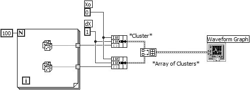
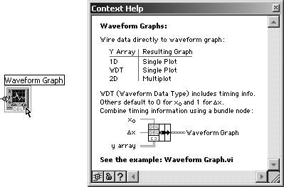
You can show more than one plot on a waveform graph by creating an array (or a 2D array) of the data types used in the single-plot examples (see Figure 8.16). Notice how graph terminals change appearance depending on the structure of data wired to them (array, cluster, array of clusters, etc.) and the data type (I16, DBL, etc.).

Figure 8.16. Passing a 2D array to a Waveform Graph to display two plots (plots are in rows of the 2D array and points are in columns)

Figure 8.16 assumes that the initial X value is 0 and the delta X value is 1 for both arrays. The Build Array function creates a 2D array out of two 1D arrays. Notice that this 2D array has two rows with 100 columns per rowa 2 x 100 array. By default, graphs plot each row of a 2D array as a separate waveform. If your data are organized by column, you must make sure to transpose your array when you plot it! Transposing means simply switching row values with column values; for example, if you transpose an array with three rows and ten columns, you end up with an array with ten rows and three columns. LabVIEW makes it easy to do thissimply pop up on the graph and select Transpose Array (this menu option is grayed out if the graph does not have a 2D array wired to it). You can also use the Transpose 2D Array function found in the Array subpalette of the Functions menu.

In Figure 8.17, the X₀ value and ΔX (or delta X) value for each array is specified. These X parameters do not need to be the same for both sets of data.

Figure 8.17. Building an array of single plot (Xo, dX, and Y array) clusters to create a multi-plot

Remember to use the Context Help window to view the detailed description of the data types that may be wired to a waveform graph (as shown in Figure 8.18). This is a very useful reference. Simply hover the mouse over the graph terminal, on the block diagram, and a detailed description of the plot data types will appear in the Context Help window. The Context Help window can be made visible by selecting Help>>Show Context Help from the menu or by using the shortcut key <control-H> (in Windows), <command-H> (in Mac OS X), or <meta-H> (in Linux).