Monitoring Disk IO
Monitoring Disk I/O
Disks are an important part of any server platform. Used for the storage of your logs, application data, database files, binaries, and even swap space, their speed is a key input to your platform's overall performance.
You'll now look at how to diagnose "hot" disks and determine their utilization. It's worth highlighting that many high-end disk vendors (for example, vendors that produce controllers and disks, external arrays, and the like) quite often supply software that provides monitoring capabilities for their specific products.
In most cases, if your disks are host connected, then you'll be able to use the standard Unix and Windows tools discussed in this chapter, as well as the proprietary vendor software.
Disk I/O: Unix
Disk I/O in Unix follows a fairly standard design and is somewhat common between all Unix flavors. As discussed in earlier chapters, hard disks are limited by a range of factors that depict their so-called performance level. To summarize, a disk's performance is gauged by a number of factors that, when combined, produce a maximum and sustained transfer rate as well as a maximum and sustained I/O rate. What makes up these factors is everything from rotational speed, onboard cache memory, control and architecture type, and the way in which the data is written to disk.
You can use a number of commands on the three Unix-like platforms discussed throughout this book. The most common one is the iostat command. The iostat command is a common Unix application available on AIX, Linux, and Solaris that provides an ability to understand what's going on within the disk subsystems.
| Note | The iostat command has many different display and output options. The options used here provide the best all-around results. However, you may find that other parameters suit your environment better. |
The following is some sample output from an iostat command:
~>iostat -xnM extended device statistics r/s w/s Mr/s Mw/s wait actv wsvc_t asvc_t %w %b device 4.0 2.9 0.0 0.0 0.0 0.0 2.3 4.0 0 2 c0t0d0 6.7 5.0 0.0 0.0 0.0 0.1 1.4 11.7 1 8 c0t2d0 0.0 0.0 0.0 0.0 0.0 0.0 8.3 153.2 0 0 c0t3d0
What this command output shows you is a Unix server ( specifically , Solaris) that has three disks attached to it (note the three targets, each with a single disk on them in the device column).
Looking at the key data elements on the output, you can tell that the first disk is servicing about seven I/Os per second. You can draw this from adding the r/s , or reads per second, and the w/s , or writes per second, columns .
The next two columns refer to the sum of data transferred ”read or written. This is a helpful indicator if you suspect that your Small Computer System Interface (SCSI), Advanced Technology Attachment (ATA), Integrated Device Electronics (IDE), or Fibre Channel bus is running out of bandwidth. By summing up these two columns for all disks on the same bus, you can get an approximate total bus transfer rate.
The next column, wait , refers to how many I/O requests are queued. It's possible to use this number and understand how much the response time of the disks are contributing to the queuing of I/O request.
The next column, actv , shows the number of active I/Os taken off the I/O queue in the time frame of the command's run and processed .
The next two columns, wsvc_t and asvc_t , are the average response time for I/Os on the wait queue and the average response time for active I/Os, respectively.
The last column of interest is the %b column. This infers the overall utilization of that particular disk. In the previous example output, the first disk is only 2 percent utilized, the second 8 percent, and the third 0 percent.
Picking a Hot Disk
Using the iostat command, you're able to identify where a specific disk may be performing badly within your environment and may be impacting overall performance.
A hot disk could be the cause of poor performance within a WebSphere application environment if there's a lot of disk I/Os occurring, such as I/Os to an application log file or reading dump data. Another cause of a high disk I/O is constant or high use of swap space by your operating system. The most obvious sign of a hot disk is the %b column. If it exceeds 50 percent, then your disk will start to become a bottleneck.
The first two columns that refer to the reads and write I/Os per second should also be considered as a guide. As mentioned in Chapter 5, generally , for SCSI and Fibre Channel disks, you can extract 10 I/Os per second from the disk for every 1,000 Revolutions Per Minute (RPM) that the disk can produce. That is, for a 10,000RPM SCSI disk, you can work on achieving 100 I/Os per second. A 7,200RPM SCSI disk will provide you with approximately 70 I/Os per second. As also discussed in Chapter 5, the way to get beyond these I/O limitations is to stripe your disks.
In the previous example, these drives are specifically 7,200RPM drives . The I/O rate for the second drive is approximately 12 I/Os per second. This equates to approximately 17 percent utilization of the disk. However, you'll see that the %b column only says 8 percent utilization. What this means is that although there are 12 I/Os per second occurring, the size of the I/Os are very small and there's an additional amount of headroom available.
Another key performance indicator is the response time and depth of queued I/Os. The actv , or the number of active I/Os taken off the queue (to be processed), should be no more than 1. Generally speaking, this field will become close to 1 as the %b field, or disk utilization, nears 50 percent ”give or take.
Table 13-1 summarizes the key hot disk indicators and what they mean in terms of negative disk performance.
| Measurement | Meaning | Fix |
|---|---|---|
| Asvc_t field greater than 30 milliseconds (ms) | As the number of I/Os increases, the response time to perform I/Os to the particular disk increases . | Redistribute load over disks, purchase faster disks, or consider striping. |
| Act_v greater than 1 | As the number of I/Os queues up, this element will increase. A rate of 1 corresponds approximately to 50 percent of %b . | Redistribute load over disks, purchase faster disks, or consider striping. |
| %b greater than 50 | %b shows the average utilization of the disk I/O to this particular device. This takes into consideration all the previous measurements as well as the number and frequency of writes and reads per second. | Redistribute load over disks, purchase faster disks, or consider striping. |
Disk I/O: Windows NT/2000/XP
Disk performance in a Windows server environment has the same implementation considerations as for Unix. Striped disks are always the key in distributing load off single spindles, and this is no different for Windows servers. Similar to monitoring the CPU utilization, monitoring the performance of disks within a Windows server can be done via the Performance tool.
From the details in the previous sections about CPU and system utilization, you know you can open the Add Counters dialog box and select various disk monitoring options.
| Note | The details discussed in the Unix section (such as I/O rates, disk utilization, and limitations) are all applicable to a Windows world. The disks, and in many cases the controllers, are the same (there are just specific driver differences). |
The types of disk performance indicators you want to monitor are the same as for the Unix world:
-
Queue Length: How many I/Os are waiting on the queue
-
% Disk Time: How much time is the disk(s) taking to service the I/O requests
In the Unix section, you learned about the iostat tool. Many of the same iostat outputs ”such as reads and writes per second, read and write kilobytes/megabytes per second, and so forth ”can all be modeled using the system performance tools.
In the Add Counters box, you want to add the two settings, Queue Length and % Disk Time, from the counters list. Once these are selected and your desired disks are being captured (remember, you can add those two options for multiple disks), close the dialog box to start the monitoring.
Figure 13-6 shows graph depicting a Windows XP-based server, charting both Queue Length and % Disk Time.
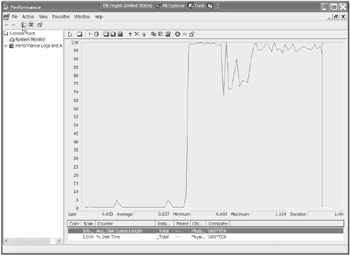
Figure 13-6: Graphing Queue Length and % Disk Time
The important points to monitor here are that the % Disk Time counter shouldn't be more than 50 percent over long periods and the Queue Length counter should remain less than 1 for 75 “85 percent of the time. High bursts are fine as long as they don't constitute the norm and don't exceed 15 “25 percent as a maximum.
EAN: 2147483647
Pages: 111