5.2 Primitive Measures of Source Code

5.2 Primitive Measures of Source Code

Before discussing the process of measuring source code, it will be useful for us to identify precisely what our objectives are in doing so. There are really two different aspects of a program when a developer writes it. First, the developer must interact with the programming language metaphor. Second, the developer must specify the actions that the code will take at runtime. In C++, for example, a developer must come to grips with the notion of objects and their instantiation. At runtime, however, a program is nothing more than an ordered sequence of machine-level instructions. The programming language metaphor will vanish when the code is compiled. The real value in measuring aspects of the programming language metaphor has to do with the interaction of this metaphor with the developer's psychological attributes. We choose, in this chapter, to discuss only those code attributes that persist through the compilation and result in actual machine code. This is not because we do not regard the measurement of attributes of the language metaphor as important. They are. Most of our recent work has focused on the software that it actually executing. Therefore, we admit to a distinct bias in measuring those source code attributes that persist at runtime.

As established in Chapter 3, we will conduct all of our measurements on program modules. The notion of a module, of course, will vary from one programming language to another. In the case of the C programming language, the choice is simple. A module is a C function. The measurements for a program, then, will be the sum of the modules of a program. That is, if we have a program consisting of five modules, each of which has exactly 100 lines of code (whatever that might mean), then the program will have exactly 500 lines of code in it.

The basis of Halstead software science metrics was that a compiler would process the source code to produce an object program. ^[12] In the process of doing this, the compiler would have to resolve all tokens established during the process of lexical analysis into one of two distinct classes. A token is an operator or it is an operand. Further, each of these counts for a program could be tallied in two distinct ways: total operators (operands) and unique operators (operands). All other metrics would be derived from these primitive measures.

Our research has shown that Halstead's primitive measures of operator and operand count account for substantially all of the variability among programs in the set of Halstead software science metrics. ^[13] That is, there is little or no information in the measures of program vocabulary, effort, etc. What is important about Halstead's work in metrics is the fact that the metrics were derived from the language constituents that the compiler would work with to transform the program from a higher-level language to the appropriate machine code. Very simply, the higher-level language was an intermediate representation of the operations necessary to solve a computational problem on a computer. Higher-level language abstractions would be transformed into sequences of code to operationalize these concepts.

We think that this approach is a very good idea. Very little is known about the psychological processes that surround the act of programming. Metrics based on elementary mental discriminations made by the programmer are suspect at best. On the other hand, quite a bit is known about how compilers transform higher-level language abstractions into machine code. Constructs and activities in this process are quite measurable.

5.2.1 Measures of Program Size

Software developers and testers are often required to measure software attributes to control, predict, or manage the software process and the software products. Although suggestions might be found regarding the measurement of source code, there is not a set of precise definitions or standards to evaluate source code attributes for any language. The National Institute of Standards and Technology does not deem this standardization to be within its purview. The conflict that arises from the lack of standards is that different measurement tools produce different values for the same program attributes for identical programs. In essence, each measurement tool developer is defining his own de facto metric standard. Most metric tool developers are very careful not to disclose the precise method of enumeration by which metric values are obtained by their tools, almost as if a trade secret would be disclosed by such a revelation.

In essence, it is not possible in the current environment to conduct scientific inquiry into any investigations involving source code measurement. We can build our measurement tools to conduct our own private inquiries, but we certainly cannot share these results in the scientific literature. For there to be science, there must be repeatability of results. It is of little or no value to us to learn that the average program module size as reported in the literature was, say, 150 statements. There are no clear rules for the enumeration of statements. We will never be able to reproduce even the simplest investigation because we are all using different rulers for our measurements.

5.2.1.1 Compiler Directives.

Our stated measurement objective will be to measure source code attributes that persist through the compilation process to execution. Therefore, all compiler directives must be resolved before the measurement process can begin. The rationale for this is quite simple. The include compiler directive can dump several hundred lines of code into a program module when it is resolved by the compiler preprocessor in charge of these things. Very simply, the measurement process can be applied only to post-processed source code. None of our measurements will be taken on compiler directives. They must be resolved, not measured, before the source code measurement process can begin. They are part of the programming language metaphor.

There is very little real science in the literature on programming language practice. There is clear evidence that global variables are bad programming practice. They are bad because a significant number of the total fault population for a given program will be attributable to errors by developers in changing the values of these variables. In the C programming language, we will choose to treat global variables as if they are compiler directives. All global definitions will be mapped into the individual program modules within the scope of the definitions.

5.2.1.2 Style and Statement Metrics.

A programmer may have a strong influence over the manner in which a program is constructed. Some programmers use many comment statements to document their activities. Other programmers think that their code must be self-explanatory. Some programmers tend to write very short statements while others might implement the same design specification in very few lines (which generally creates a particular type of C code known as write-only code). Some programmers are very terse in their use of declarations. Other programmers will be very expressive with their use of declared variables. The first class of metrics we wish to define are those that relate to the frequency of use of comments, executable program statements, and nonexecutable statements.

Comments can be represented in many different ways in various programming languages. In some languages, they must be on a separate line by themselves. In others, they may be embedded in a line containing executable code. The rules for comments vary considerably. In the C programming language, we will identify a comment by the token triple </*> <string> <*/>. Each occurrence of this token triple will cause our Comment metric to be incremented by one. Global comments will not be counted. For example, in the C programming language it is possible to put multiple C modules (functions) into one file. Comments can be placed anywhere in this file. We will choose to ignore those that are not physically contained in a program module. We are interested in enumerating only comments that are specific to a particular module. Global comments do not meet this criterion; they are clearly outside the scope of any function module.

Enumerating the number of comments in a programming language is not necessarily a meaningful exercise. Developers tend to put comments into code because they have been told to do so and their compliance with this requirement will be measured by the Comment metric. If a program module is designed correctly, it will contain no comments at all. Each program module should reflect exactly one design element. This design element will partially implement a particular functionality. Thus, the documentation for a program module should be maintained in the design, and not in the code. The name of the developer and the names and dates of the subsequent developers and program modifications should be maintained by the configuration control system. This leaves little or no reason for commented code.

Perhaps the most common program attribute being measured today is the number of lines of code, LOC, in a program. This metric is used everywhere and formally defined nowhere. A very simple definition of LOC in the UNIX environment is the number of logical records in a source code file. In the case of UNIX, a logical record is delimited by <CR>. If we choose to measure LOC in this manner, it will automatically include the number of lines that contain comments only. It will also include lines that contain only white spaces, which in the UNIX environment are <SPACE> and <TAB>. If we are using LOC as a measure of programmer productivity, a wise programmer will be sure to include plenty of comments and blank lines in his program. Perhaps the best way to count LOC is to eliminate lines that contain only comments and lines that contain only white spaces. If we choose to enumerate LOC prior to invoking the compiler preprocess to resolve the compiler directives, LOC will reflect these compiler directives which represent a dialog between the programmer and the compiler. If we want to enumerate LOC after the preprocessor has been invoked, then we find that the preprocessor has taken some serious liberties with the number of logical source records in the post-processed code. In either case, LOC is one of the most misleading measurements that we could hope to get on a program. As a measure of size it can be misleading. We might potentially learn the wrong thing about what we seek to know through the use of this metric.

Another metric that clearly contributes to our confusion about the actual size of a program is the KLOC metric. When we are measuring the number of memory locations in a computer system, the prefix "K" clearly means 2¹⁰ (or 1024). In most cases when someone reports that her program is 10 KLOC, the value of K is probably 10³ (or 1000). This is a small point. These two values differ by only about 2 percent. The obfuscation possible in the determination of LOC is certainly much larger than this.

The next program size attribute that we would like to measure is the number of executable statements, which we will denote by the Exec metric. This is a very difficult attribute to define and to measure. We can measure it in any number of ways. The fact that there are many different ways to measure Exec does not mean that it is of no value. What is important is that we specify exactly how we choose to measure it and report this unambiguously. We will, of course, meet this ambiguity criterion if a colleague in another part of the world can measure the same source code that we measured and get exactly the same result.

For our measurement of the Exec attribute, we will require that the source code artifact being measured actually change the state of the machine at runtime in order for a statement to increment the statement count. It is clear that the statement

• count = count + 1;

is an executable statement. It is also clear that:

• int a;

is not an executable statement. It is not completely clear whether

• int a = 1;

is executable. If the integer a is to receive a value of 1 whenever the block containing the declaration is entered, then this is clearly an executable statement and the Exec count is incremented by one when this statement is encountered. The runtime effect of each statement within a programming language metaphor must be carefully examined to prepare the rules for the computation of Exec.

Sometimes, we really do not know what will happen to certain constructs such as the initialization example above. This is particularly true of the C++ metaphor. The syntax for C++ is fraught with ambiguities, and the semantics of the language are more or less at the mercy of the group who wrote each C++ compiler. Thus, many times, we will be forced to create test cases to determine just how the system works. The question at hand is, in the construct

• int a = 1;

does the variable a get its value from the compiler at compile time or is it reset at runtime? If a receives a new value every time the block that contains this declaration is entered at runtime, then this declaration should be enumerated as an executable statement.

Because we really do not know the answer to this question, let us conduct a test. Consider the following C program:

      main()      {        void test (void);        test();        test();      }      void test(void)      {        int i = 0;        i++;        printf ("%d \n," i);      } 

If the compiler initializes the location i to 0 during compilation, then the program should print first 1 and then 2. When we run the program, we find that it prints 1 and then 1. It is now obvious that the initialization is taking place at runtime. Thus, this declarative statement must be counted as an executable statement.

In general, the character ";" is used to delimit statements in the C programming language. The Exec metric is incremented by one every time a semicolon is found at the end of a statement that has been identified as executable. This is not always clearly the case. Consider the following for statement:

     for (i = 1; j = i<50; i++) k + = j; 

There are clearly four executable statements within this one construct. They are:

    1. i = 1    2. j = i<50    3. i++    4. k + = j 

Three of these statements are delimited by semicolons. One (i++) is delimited by the token <)>.

Now consider the following program segment from a C program module:

    i = j + 1;    {      int a = 1, b = 1;      k = a + b + I;    } 

Now it should be clear that there is yet another statement delimiter. It is the token <,>. The statement delimited is:

    a = 1 

in that it is clear to us from our previous example that this declaration is, in fact, executable.

A statement, so far, can be delimited by the tokens <;>, <)>, and <,>. But, we are not finished yet. It turns out that a compound statement delimited by <{> and <}> is also a statement. There are two types of compound statements: those with declarations in them (blocks) and those without. The difference is that a block will create an activation record when it is entered at runtime. It has execution consequences. A compound statement merely brackets statements for the compiler. The braces have no runtime consequences. Thus, the program segment shown above should increment the Exec count by five.

The rules for counting statements can be very complicated. In some programming language metaphors such as C++, the rules for counting statements are astonishingly complex. Unless we have access to the precise set of counting rules, we do not really learn much when they report to us that they have a C program containing 100 statements. We have included in Appendix 2 a standard for the measurement of statements in the C programming language. The purpose of including this standard is that it is a reference point. If a metrician wishes to enumerate certain constructs differently, he need only reference this standard and indicate the modifications that he has made to it. The real role of this standard is to serve as a reasonable template for the creation of similar standards for the C programming language and other programming languages. Maybe if we as an emerging science are lucky, the National Institute of Standards and Technology will choose to embrace software measurement technology as well, and then set and maintain these standards.

Nonexecutable statements represented by the metric NonExec are present in variable declarations, structures, unions, enumerated declarations, and type definitions. If a variable is declared, the declaration is considered a nonexecutable statement. It should now be clear that in languages derived from Algol, compound statements are nonexecutable statement and will cause NonExec to be incremented, whereas blocks will cause Exec to be incremented. If a statement does not modify the runtime environment in any way, then it will be a nonexecutable statement. Comments are not nonexecutable statements. Some sample code and how nonexecutable statements are enumerated can be seen in Exhibit 1. Most notable in this exhibit is the construct int i = 3 ;. This single statement is really two distinct statements. There is a nonexecutable component, int i; and there is an executable component, i = 3 ;.

Exhibit 1: Nonexecutable Statements

Example	Nonexecutable Statement
int i; int i = 3 ; typedef int bool; struct time { int hour; int minute; }; typedef struct time { int hour; int minute; } timetype; timetype a, b, *c;	1
	1
	1
	3
	4

5.2.2 Lexical Metrics

The lexical analysis of a source program module in any language will resolve the strings of characters on the input stream to a sequence of tokens. We can assign the elements of the set of tokens obtained from this lexical analysis of a program module into two mutually exclusive sets. Some tokens will cause action to be taken by the compiler either at compile time or at runtime. These tokens will be called operators. Other tokens represent the operands of the individual operators. These categories were first measured by Maurice Halstead. ^[14]

There are two distinct ways to enumerate both of the categories of operators and operands. We can count the total times that a particular operator or operand has been used. That is, we can measure the number of operators (or operands) by the cardinality of the set of all operators (operands) found during the lexical analysis of a source program. Alternatively, we can measure the number of distinct operators (operands) by the cardinality of the set of unique operators. Comments are not considered to be either operators or operands.

The count of total operators for a program was denoted by N₁ by Halstead and the total operand count by N₂. This is now fairly standard nomenclature. When Halstead originally conceived these metrics, he thought to apply them only to arithmetic expressions within a program. We are going to stretch the definition a bit of both operator and operand to a much more general case so as to cover all tokens in a program, not just those in arithmetic expressions. Consider the following C program:

    main ()    {      int a, b;      a = 1;      b = 2;      b + = a;      printf (%d, b);      exit;    } 

There are 30 total tokens in this program; they are as follows:

    <main>, <(>, <)>, <{>, <int>, <a>, <,>, <b>, <;>, <a>, <    = >, <1>, <b>, < = >, <2>, <;>, <b>, <+ = >, <a>, <;>,    <printf>, <(>, <%d>, <,>, <b>, <)>, <;>, <exit>, <;>, and    <}>. 

We can now divide this set into the set of operators O_l and the set operands O₂. The set of operators is:

     O1 = {<main>, <(>, <)>, <{>, <int>, <,>, <;>, < = >, <;>,    <+ = >, <;>, <printf>, <(>, <,>, <)>, <;>, <exit>, <;>,    <}>} 

There are 20 operators. We would say that N₁ = ||O₁|| = 20 for this program. The set of operands is:

    O2 = {<main>, <a>, <b>, <a>, <1>, <b>, <2>, <%d>, <b>, <a>,    <printf>, <b>, <exit>} 

Thus, there are 13 operands and N₂ = ||O₂|| = 13.

It is interesting to note that the sum of N₁ and N₂ is not equal to 30. This is so in that the intersection set of operators and operands contains the tokens for the three function calls: <main>, <printf>, and <exit>. This is an interesting aspect of the C programming language. Each function call returns a value. Thus, <printf> is at once an operator (function call) and an operand (it contains a return value).

The set of unique operators O₃ is:

      O3 = {<main>, <(>, <) >, <{>, <int>, <,>, <;>, < = >, <+ =      >,  <printf>, <exit>, <}>} 

The number of unique operators, η₁, is equal to the cardinality of the set O₃. Thus, η₁ = ||O₃|| =12. The set of unique operands is:

      O4 = {<main>, <a>, <b>, <1>, <2>, <printf>, <%d>, <exit>} 

The number of unique operands, η₂, is equal to the cardinality of the set O₄ and η₂ = ||O₄|| = 8.

In a language such as C, an operator may be overloaded. That is, it may be called to serve many different duties. Take, for example, the operator <+>. This operator can be used for integer operands or for real operands. Further, it can be used as a unary operator or as a binary operator. In each of these roles it is doing different duty. Consider the case where <+> is infixed between two integer operands a + b. The compiler will generate the code for the two operands, a and b, to be added together using binary integer arithmetic. If, on the other hand, a and b are both real operands, then the compiler must generate the code for the two operands to be added using floating point arithmetic. The single operator <+> can be used in the following contexts in the C programming language.

As a binary operator:

+	+1	integer
+	+2	short
+	+3	Long
+	+4	Float
+	+5	double

As a unary operator:

+

+₆

all operands

We will not be able to distinguish among these many different contexts during the lexical phase. Indeed, we will only be able to distinguish an integer addition from a floating addition when we have achieved binding between type and each of the operands. Once we are able to type to operands, we can then identify a new metric, η₃. Halstead did not choose to deal with the problem of overloading; he counted only the total operator tokens. We have found this to be incomplete. A C program is far richer in operands, in terms of their runtime consequences, than the η₂ metric would indicate. η₃ is the number of unique operators in a program accounting for overloading. That is, we will count a +₄ b as a floating operation, where a and b are floating point operands. This will differentiate the operator in the expression i +₁ j, where i and j are integer operands. An example of the enumeration of the η₃ metric is shown in Exhibit 2.

Exhibit 2: Unique Operator—Operand Counts

Example	η1	η3
{ int i1 = 1,i2 = 2,i3; float f1 = 1.1, f2 = 2.2, f3; i3 = i1 + i2; f3 = f1 + f2; }	8 unique overloaded operators: { int = , ; float + }	10 unique operators: { int = 1 , ; float = 2 +1 +2 }

5.2.3 Control Flowgraph Metrics

The internal structure of a program module will have a great effect on the number of potential faults it might harbor. A module that contains a lot of statements but no predicate clauses (such as in if statements) will be very easy to understand and to program. It will present little opportunity for the designer or developer to stray from the straight line. Another program module with fewer statements but a really complex control structure will offer both the designer and the developer plenty of opportunity to introduce faults. We will model the internal structure of a program module in terms of its control flowgraph.

A control flowgraph of a program module is constructed from a directed graph representation of the program module that can be defined as follows:

• A directed graph, G = (N, E, s, t), consists of a set of nodes, N, a set of edges E, a distinguished node s the start node, and a distinguished node t the exit node. An edge is an ordered pair of nodes (a, b).

• The in-degree I(a) of node a is the number of entering edges to a.

• The out-degree O(a) of node a is the number of exiting edges from a.

The flowgraph representation of a program, F = (E', N', s, t), is a directed graph that satisfies the following properties:

• There is a unique start node s such that I (s) = 0.

• There is a unique exit node t such that O (t) = 0.

• We will represent both the start node, s, and the terminal node, t, by the symbol . All other nodes, n←N', are members of exactly one of the following three categories:

  1. Processing node: It has one entering edge and one exiting edge. They represent processing node a, I (a) = 1 and O (a) = 1. In our diagrams we will represent a processing node as .

  2. Predicate node: Represents a decision point in the program as a result of if statements, case statements, or any other statement that will cause an alteration in the control flow. For a predicate node a, I(a) = 1 and O(a) > 1. We will represent this by the symbol .

  3. Receiving node: It represents a point in the program where two or more control flows join, for example, at the end of a while loop. For a receiving node a, I(a) > 1 and O(a) = 1. This will be represented by the symbol .

• A set of edges E' connecting the elements of N'.

If (a, b) is an edge from node a to node b, then node a is an immediate predecessor of node b and node b is an immediate successor of node a. The set of all immediate predecessors for node a is denoted as IP(a). The set of all immediate successors for node b is denoted as IS(b). No node may have itself as a successor. That is, a may not be a member of IS(a). In addition, no processing node may have a processing node as a successor node. All successor nodes to a processing node must be either predicate nodes or receiving nodes. Similarly, no processing node may have a processing node as its predecessor.

From this control flowgraph representation, two essential control flow primitive metrics emerge:

1. Number of nodes

2. Number of edges

A path P in a flowgraph F is a sequence of edges, , where all a_i (i = 1,...,N) are elements of N'. P is a path from node a₁ to node a_N. An execution path in F is any path P from s to t.

The average length of the paths measured in numbers of edges constitutes a second program characteristic. A program that has a large number of relatively short control-flow paths differs greatly in terms of testing or maintenance from one having a few relatively long control-flow paths.

Another very important feature of a flowgraph, the representation of program iteration constructs, must be considered. A program may contain cycles of nodes created by if statements, while statements, etc. These iterative structures are called cycles as opposed to the more familiar concept of a programming loop. A loop is simply a cycle of length one (containing one node and one arc). Whether the nodes lie on a cycle relates to the concept of connectedness defined as follows:

• A flowgraph F is weakly connected if any two nodes a and b in the flow-graph are connected by a sequence of edges.

• A flowgraph F is strongly connected if F is weakly connected and each node of F lies on a cycle.

As an aside, all flowgraphs are only weakly connected in that the start node has an in-degree of zero and the exit node has an out-degree of zero. However, a flowgraph may be made strongly connected by inserting an edge, (t, s), connecting the exit node with the start node.

Any flowgraph can potentially contain weakly connected subsets of nodes that are flowgraphs in their own right. To examine this potential hierarchical structure of the flowgraph representation, the notion of a sub-flowgraph is essential.

• A subflowgraph F' = (N", E", s', t') of a flowgraph F = (N', E', s, t) is a flowgraph if the out-degree of every node in F' is the same as the out-degree of the corresponding node in F with the exception of the nodes s' and t'. Further, all nodes in the subflowgraph are weakly connected only to nodes in N".

• A subflowgraph of F is a subflowgraph with the property that the cardinality of N" > 2 and F' ≠ F. That is, the subflowgraph must contain more nodes than the start and exit nodes and cannot be the same flowgraph.

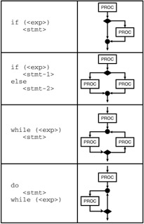
A flowgraph is an irreducible flowgraph if it contains no proper subflowgraph. A flowgraph is a prime flowgraph if it contains no proper subflowgraphs for which the property I(s') = 1 holds. A prime flowgraph cannot be built by sequencing or nesting of other flowgraphs and contains a single entrance and a single exit structure. The primes are the primitive building blocks of a program control flow. In the C language, the prime flowgraphs are the basic control structures shown in Exhibit 3.

Exhibit 3: Prime Flowgraphs

The total path set of a node a is the set of all paths (s, a) from the start node to the node a itself. The total path count of a node a is the cardinality of the path set of the node; hence, each node singles out a distinct number of paths to the node beginning at the start node and ending with the node itself. The path count of a node simply equals the number of such paths.

Now that we have constructed a practical means of discussing the internal structure of a program module, we will use this methodology to create a program flowgraph for each program module and then enumerate certain characteristics of the flowgraph to represent the control complexity of the corresponding program module.

Converting a C program into its flowgraph representation is not an easy task. We would like to do this in such a manner that the flowgraph we generate from a program would be determined very precisely. That is, any person building a metric tool and following our rules will get precisely the same flowgraph that we would.

First, we will establish that the predicate nodes and the receiving nodes represent points on the flowgraph. That is, they do not represent any source code constructs. All source code will map to the processing nodes.

Because of the complexity of the C grammar, we must decompose switch statements into their component parts before the flowgraph can be constructed accurately. Consider the following C code segment:

      switch (<exp>)      {        case <c_exp1> : <stmt>;        case <c_exp2> : <stmt>;        case <c_exp3> : <stmt>;        default : <stmt>;      } 

This switch statement is functionally equivalent to the following decision structure:

    if (<exp> =  = <c_exp1>)      goto lab1;    if (<exp> =  = <c_exp2>)      goto lab2;    if (<exp> =  = <c_exp3>)      goto lab3;    else      goto lab4;    lab1: <stmt>;    lab2: <stmt>;    lab3: <stmt>;    lab4: <stmt>;    lab5: 

Similarly,

    switch (<exp>)    {      case <c_exp1> : <stmt>;      break;      case <c_exp2> : <stmt>;      case <c_exp3> : <stmt>;      default : <stmt>;    } 

is equivalent to

    if (<exp> =  = <c_exp1>)      goto lab1;    if (<exp> =  = <c_exp2>)      goto lab2;    if (<exp> =  = <c_exp3>)      goto lab3;    else      goto lab4;    lab1: <stmt>;      goto lab5;    lab2: <stmt>;    lab3: <stmt>;    lab4: <stmt>;    lab5: 

This new structure is essentially the control sequence that a compiler will generate for the switch statement. It is not pretty. The moral to this story is that switch statements are probably not a good idea. Nested if statements are probably better alternatives.

There are other unfortunate constructs in C that have an impact on the control flow of a program. Expressions that contain the logical operator && are, in fact, carelessly disguised if statements. Consider the following C code, for example:

     if (d > e && (b = foo (zilch))       <stmt>; 

It is clear that the function foo may or may not get called and that b, as a result, may or may not have its value changed. Thus, whenever we find the logical product operator &&, we must break the predicate expression into two or more if statements as follows:

     if (d > e)       if (b = foo (zilch))     <stmt>; 

The same fact is true for the conditional expression. If we were to find the following C code

     c = a < b ? 5 : 6; 

we would rewrite this as:

     if(a < b)       c = 6;     else       c = 7; 

to determine the appropriate flowgraph structure for this conditional expression.

For the sake of simplicity, we will temporarily set aside the rule that a processing node cannot have a processing node as its own successor. We will use this rule to refine the control flowgraph once we have a working model. The following steps will build the initial flowgraph.

1. The opening brace <{> and any declarations in a function will automatically constitute the first processing node of the flowgraph. The first node, of course, is the start node, which represents the function name and formal parameter list.

2. Each expression or expression statement will generate a processing node linked to the previous node.

3. All labels will generate a receiving node.

4. All expressions in selection statements (<if> and <switch>) will be extracted from the parentheses and will constitute one processing node that precedes the predicate node of the selection itself.

5. The <if> and <switch> will be replaced with a predicate node linked immediately to the next processing block.

6. In the case of the iteration statement <while>, three nodes will be generated. First is a receiving node to which control will return after the execution of the statement following the while expression. Next, the expression will be extracted and placed in a processing node. Finally, the predicate node will be generated and linked to the next processing node and to the next statement after the while group. The last processing node in the structure will be linked to the receiving node at the head the structure.

7. In the case of the <for> iteration statement, the first expression in the expression list will be replaced by a processing node followed by a receiving node, and the second (and third) expression(s) will be replaced by a processing node.

8. The <for> token will be replaced with a receiving node linked to the next processing node.

9. The <do><while> statement will have its predicate node following the statement delimited by <do> and <while>. First, the <do> token will be replaced by a receiving node that will ultimately be linked to the end of the do-while structure.

10. The statement following the <do> token, together with the expression after the <while> token, will be grouped with the do statement.

11. A <goto> statement implies the existence of a labeled statement. All labels will be replaced with receiving nodes. The effect of the <goto> is to link the current processing block containing the <goto> to the appropriate receiving node.

12. The <continue> and <break> statements are, in effect, <goto> statements to the unlabeled statement at the end of the control structure containing them.

13. All <return> statements will be treated as if they were <goto> statements. They will link to a receiving node that immediately precedes the exit node. If there is an expression associated with the return statement it will create a processing node that is, in turn, linked to the penultimate node. If there is but one return and it is at the end of the function module, then this receiving node with but one link will be removed in the refinement stage.

14. All assignment statements and expression statements will generate one processing node.

15. The declaration list of any compound statement will generate one processing node, which will also contain all executable statements in the declaration list.

After the preliminary flowgraph has been constructed by repetition of the above steps, it can then be refined. This refinement process will consist of:

• Removing all receiving nodes that have but one entering edge

• Combining into one processing node all cases of two sequential processing nodes

When all remaining nodes meet the criteria established for a flowgraph, its structure can be measured.

Exhibit 4 shows a sample C program. The first column of this exhibit shows the original C program. The second column shows the decomposition of this program according to the rules above. In this example, the nodes have been numbered to demonstrate the linkage among the nodes.

Exhibit 4: Sample Program Decomposition

 int average(int number) {     int abs_number;     if (number > 0)         abs_number = number;     else         abs_number = -number;     return abs_number; } 

 < 0 START NODE int average(int number)> < 1 PROCESSING NODE {    int abs_number; LINK 2> < 2 PROCESSING NODE (number > 0) LINK 3> < 3 PREDICATE NODE if LINK 4, 5> < 4 PROCESSING NODE abs_number = number; LINK 7> < 5 RECEIVING NODE else LINK 6> < 6 PROCESSING NODE abs_number = -number;    LINK 7> < 7 RECEIVING NODE LINK 8> < 8 PROCESSING NODE abs_number;return LINK 9> < 9 RECEIVING NODE LINK 10> < 10 EXIT NODE}> 

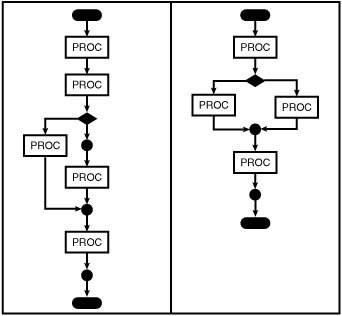
In Exhibit 5, there are two figures. The figure on the left shows the graphical representation of the initial program decomposition. This is not a flowgraph. We can find, for example, two processing blocks in a row. There is also a receiving node with one entering edge and one exiting edge. When the surplus processing blocks are combined and the unnecessary processing block removed, we get the final flowgraph shown by the figure on the right in this exhibit.

Exhibit 5: Reduction of the Flowgraph

The Nodes metric will enumerate the number of nodes in the flowgraph representation of the program module. The minimum number of nodes that a module can have is three: the start node, a single processing node, and the exit node. Although it is possible to create a module with just the starting node and a terminal node, it does not make sense for a real system. Modules with just two nodes can be part of a testing environment as stubs but they should not be present in a deliverable product.

If a module has more than one exit point (return), then a receiving node must be created to provide for a single exit node for the structure. This receiving node will ensure that there is a unique exit node. In general, it is not a good programming process to use multiple return statements in a single program module. This is a good indication of lack of cohesion in a module.

The Edges metric will enumerate the edges in the control flow representation of the program module. For a minimal flowgraph of three nodes, there will, of course, be two connecting edges.

A path through a flowgraph is an ordered set of edges (s,..., t) that begins on the starting node s and ends on the terminal node t. A path may contain one or more cycles. Each distinct cycle cannot occur more than once in sequence. That is, the subpath (a, b, c, a) is a legal subpath but the subpath (a, b, c, a, b, c, a) is not, in that the subpath (a, b, c, a) occurs twice.

The total path set of a node a is the set of all paths (s, a) that go from the start node to node a itself. The cardinality of the set of paths of node a is equal to the total path count of the node a. Each node singles out a distinct number of paths to the node that begins at the starting node and ends with the node itself. The path count of a node is the number of such paths.

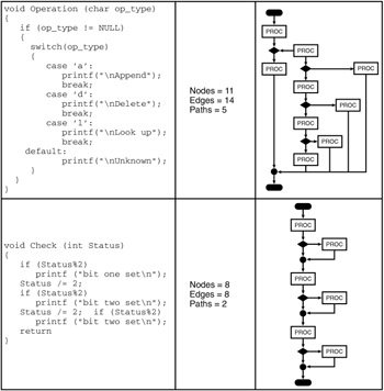
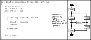
The Paths metric will tally the number of paths that begin at node s and end at node t. Sample enumeration of the Nodes, Edges, and Paths metrics can be seen in Exhibits 6 and 7.

Exhibit 6: Enumeration of Flowgraph Metrics

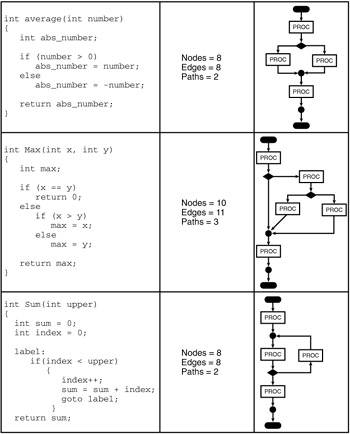
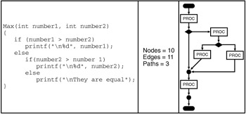
Exhibit 7: Enumeration of Flowgraph Metrics

The direct enumeration of paths in a program module may not be functionally possible. Consider the case of a simple if statement. If a program module contains but one if statement, then the number of paths doubles. In fact, the number of paths doubles for each if statement in series. We once encountered a program module that interrogated each bit in a 64-bit status word one bit at a time. This meant that there were a potential 2⁶⁴ = 18,446,744,073,709,551,616 paths through this module. If our metric tool could count 1000 paths per second in the associated control flowgraph, it would take 584,942,417 years to measure this one module. For large program modules, the number of path counts will grow very large. For our measurement purposes, our metric tools put an arbitrary path maximum at 50,000. Common sense should prevail in the design complexity of modules. We think that modules whose path count is in excess of 100 or some other reasonable value, N, should come under the scrutiny of a design review process.

Cycles are permitted in paths. For each cyclical structure, exactly two paths are counted: one that includes the code in the cycle and one that does not. In this sense, each cycle contributes a minimum of two paths to the total path count. The number of cycles in the module flowgraph will be recorded in the Cycles metric. When the path contains control logic, the path count within the module increases.

The MaxPath metric represents the number of edges in the longest path. From the set of available paths for a module, all the paths are evaluated by counting the number of edges in each of them. The greatest value is assigned to this metric. This metric gives an estimate of the maximum path flow complexity that might be obtained when running a module. In the example shown in Exhibit 8 for the Check function, there will be 2³ (or 8) paths through the structure. The path length is, of course, the number of arcs or edges that comprise the path. Thus, the length of the maximum path is 10. There is one path of length 7, one of length 14, one of length 11, and one of length 17. The average path length, Average-Path, is then 12.25.

Exhibit 8: Enumeration of Flowgraph Path Metrics

A cycle is a collection of strongly connected nodes. From any node in the cycle to any other, there is a path of length 1 or more, wholly within the cycle. This collection of nodes has a unique entry node. This entry node dominates all nodes in the cycle. A cycle that contains no other cycles is called an inner cycle. The Cycles metric will contain a count of all the cycles in a flowgraph. A sample function with a cycle in its flowgraph is shown in Exhibit 9.

Exhibit 9: An Example of the Cycle in a Flowgraph

5.2.4 Data Structures Complexity

Our own approach to the problem of measuring the complexity of data structures has been strongly motivated by the work of Halstead and our own work in the analysis of metric primitives. The basis of Halstead's software science metrics was that a compiler would process the source code to produce an object program. In the process of doing this, the compiler would have to resolve all tokens into one of two distinct classes: they were either operators or operands. Further, each of these counts for a program could be tallied in two distinct ways: total operators (operands) and unique operators (operands). All other metrics were derived from these primitive measures.

There are two broad classes of data structures: (1) those that are static and compiled with the source code, and (2) those that are created at execution time. Indeed, it is sometimes useful to model the dynamic complexity of programs. ^[15], ^[16] It is the purpose of our data structure metric to measure the complexity of static data structures. To a great extent, dynamic data structures are created by algorithms and their complexity will be indirectly measured by the control constructs that surround their creation. The data structures used in a program can influence the type of control structures used and the types of operations that can be used. The programming effort, understandability, and modifiability of a program are greatly influenced by the types of data structures used.

There is a definite difference between the complexity of a data structure as it is mapped to memory and its type complexity which are the operations that the machine will use to process data from this structure. The type properties of the structure vanish with the compilation, preserved only in the machine operations on the data. That is, the concept of type is an artifact of the particular programming language metaphor. The data structures persist at runtime. They represent real places in computer memory.

The objective of the proposed data structure measure is to obtain finer granularity on the Halstead notion of an operand and the attributes that it might have. The implementation of the notion of an operand by the author of a compiler and the operations needed to manipulate the operand (type) are two different attributes of this operand. Consider the case of an operand that is a scalar. This scalar might have a type of real or integer. On most systems, operands of these two types would occupy four bytes of memory. From the standpoint of managing the physical manifestations of each, they would be identical. The nature of the arithmetic to be performed on each, however, would be very different.

We could live a very long and happy life working with a programming language that supported only integer arithmetic. For those applications that required numbers on the interval from zero to one, we could simply use an additional integer value to store the fractional part of the number. Necessarily, performing arithmetic operations on such numbers would increase the computational complexity. The floating point data attribute greatly simplifies the act of numerical computation for real numbers. However, this type attribute will require its own arithmetic operators distinct from the integer arithmetic ones.

Thus, there appear to be many different components contributing to the complexity problem surrounding the notion of data structures. While they represent abstractions in the mind of the programmer, the compiler must make them tangible. In this regard, there are two distinctly different components of complexity. First, there is the declaration of the object and the subsequent operations a compiler will have to perform to manifest the structure. Second, there are the runtime operations that will manipulate the structure. For the purposes of domain mapping in our complexity domain model, we are interested in the operations surrounding the placement of these objects in the memory map of the object program.

Consider the several aspects of the declaration of an array in C. The declaration of an array, A, would look like this, int A[10]. A reference to the structure represented by A might include a subscript expression in conjunction with the identifier to wit: A[i]. The inherent data structure complexity represented by the subscripted variable would be represented in the increased operator and operand count of the Halstead complexity. The reference to the location, A[i], would be enumerated as two operators, <[> and <]>, and two operands, <A> and <i>. A reference to a simple scalar, say B, would count only as one operand.

The attribute complexity C(D) of a data structure D is the cost to implement a data structure. This cost is closely associated with the amount of information that a compiler must create and manage in order to implement a particular data structure while compiling a program. We would intuitively expect that simple scalar data types are less costly to implement than more complex structures. It would also be reasonable to expect that the attribute complexity of a simple integer would be less than that of a record type.

A simple, scalar data type such as an integer, real, character, or Boolean requires that a compiler manage two distinct attributes: the data type and the address. Actually, the compiler will also manage the identifier, or name, that represents the data structure. However, this identifier will be enumerated in the operand count measure. Thus, the attribute complexity, C(scalar), could be represented in a table with two entries. This structure table will contain all of the data attributes that the compiler will manage for each data structure. We define the structure by the number of entries in this structure table. Thus, the data structure complexity for a scalar will be C(scalar) = 2.

To implement an array, a compiler would require information as to the fact that it is an array, the memory location in relation to the address of the array, the type attribute of the elements of the array, the dimensionality of the array, the lower bound of each dimension, and the upper bound of each dimension. The structure table for an n-dimensional array is shown in Exhibit 10.

Exhibit 10: The Array Structure

Structure: Array

Base Address

Type

# Dimensions

Lower Bound #1

Upper Bound #1

Lower Bound #2

Upper Bound #2

•

•

•

Lower Bound #n

Upper Bound #n

In the most general sense, the computation of the attribute complexity of an array would then be governed by the formula:

• C(Array) = 3 + 2 × n + C(ArrayElement)

where n is number of dimensions in the array and C(ArrayElement) is the complexity of the array elements. For some languages, the array elements may only be simple scalars. FORTRAN is an example of such a language. In the case of other languages, such as Pascal, the array elements may be chosen from the entire repertoire of possible data structures.

Another difference can be found among languages in regard to the bound pairs of the arrays. In languages such as C and FORTRAN the lower bound of the array is fixed. The programmer cannot alter the lower bound. In this case, the compiler will not record or manage the lower bound, and the complexity of arrays in these languages will be:

• C(Array) = 3 + n + C(ArrayElement)

Other kinds of data structures may be seen as variants of the basic theme established above. For example, a string can be considered to be an array of characters. Therefore, we would compute the attribute complexity of the string as a unidimensional array. There are notable exceptions to this view. A string in language such as SNOBOL would be treated very differently. In the case of SNOBOL, there is but one data structure. Both program elements and data elements are represented as strings in this basic data structure.

A record is an ordered set of fields. In the simplest case, these fields are of fixed length, yielding records that are also of fixed length. Each field has the property that it may have its own structure. It may be a scalar, an array, or even a record. The structure table to manage the declaration of a record would have to contain the fact that it is a record type, the number of fields in the record (or alternatively the number of bytes in the record), and the attribute complexity of each of the fields of the record. The computation of the attribute complexity of a fixed-length record would be determined from the following formula:

where n is the number of fields and C(f_i) is the attribute complexity of field i.

Records with variant parts are a slightly different matter. In general, only one record field of varying length is permitted in a variant record declaration. In this case, the compiler will simply treat the variant record as a fixed-length record with a field equal in length to the largest variant field.

The attribute complexities of subranges, sets, and enumerated data types may be similarly specified. They represent special cases of array or record declarations. In each case, the specific activities that a compiler will generate to manage these structures will lead to a measure for that data type. For example, enumerated data types will be represented internally as positive integers by the compiler. Similarly, a subrange can be represented as a range of integer values, not necessarily positive. The case for sets is somewhat more complicated. A variable with a set attribute is typically represented by a bit array. Each element in the set of declared objects is represented by a bit element in this array. The size of the array is determined by the cardinality of the set.

The notion of a pointer deserves some special attention here. From the perspective of a compiler, a pointer is simply a scalar value. A programmer might infer that the pointer has the properties of the structure that it references. A compiler does not. A pointer is a scalar value on which some special arithmetic is performed. That is all. Hence, a pointer is measured in the same manner as a scalar of integer type. It has a value of 2.

The full effect of a pointer and the complexity that this concept will introduce is, in fact, felt at runtime and not at compile time. A relatively complex set of algorithms will be necessary to manipulate the values that this scalar object may receive. These values will be derived based on the efforts of the programmer and not the compiler. As a result, in this particular model, the complexity of dynamic data structures such as linked lists and trees will be measured in the control structures that are necessary to manipulate these abstract objects.

The data structures complexity of a program module is the sum of the complexities of each of the data structures declared in that module. If, for example, a program has five scalar data items, then the data structures complexity of this module would be 10, or the sum of the five scalar complexity values. If a program module were to contain n instantiations of various data structures, each with a complexity C_i, then the data structures complexity, DS, of the program module would be:

To facilitate the understanding of the calculation of the data structures metric, Exhibit 11 shows a sample C function that will serve to illustrate this process. In this very simple example, there are three declared variables, Instance, Able, and Baker. The variable Baker is an array of integers. It has a structure complexity of 6. The variable Instance is of type record. There are two fields in this record that are scalars. The structure complexity of this record is 5. The variable Able is a scalar. It is of type pointer. It has a structure complexity of 2. Thus, the DS value for this function is 13.

Exhibit 11: Sample struct Definition

       void datatest (void)       {          struct Complex {            int Fieldl;            int Field2;            } Instance;          int * Able;          int Baker [100]; 

5.2.5 Coupling Metrics

There are many different attributes that relate specifically to the binding between program modules at runtime. These attributes are related to the coupling characteristics of the module structure. For our purposes, we will examine two attributes of this binding process: (1) the transfer of program control into and out of the program module, and (2) the flow of data into and out of a program module.

The flow of control among program modules can be represented in a program call graph. This call graph is constructed from a directed graph representation of program modules that can be defined as follows:

• A directed graph G = (N, E, s) consists of a set of nodes N, a set of edges E, a distinguished node s, the main program node. An edge is an ordered pair of nodes (a, b).

• There will be an edge (a, b) if program module a can call module b.

• As was the case for a module flowgraph, the in-degree I(a) of node a is the number of entering edges to a.

• Similarly, the out-degree O(a) of node a is the number of exiting edges from a.

The nodes of a call graph are program modules. The edges of this graph represent calls from module to module, and not returns from these calls. Only the modules that are constituents of the program source code library will be represented in the call graph. This call graph will specifically exclude calls to system library functions.

Coupling reflects the degree of relationship that exists between modules. The more tightly coupled two modules are, the more dependent on each other they become. Coupling is an important measurement domain because it is closely associated with the impact that a change in a module (or also a fault) might have on the rest of the system. There are several program attributes associated with coupling. Two of these attributes relate to the binding between a particular module and other program modules. There are two distinct concepts represented in this binding: the number of modules that can call a given module and the number of calls out of a particular module. These will be represented by the fan-in and fan-out metrics, respectively. ^[17]

The F₁ metric, fan-out, will be used to tally the total number of local function calls made from a given module. If module b is called several times in module a, then the F₁ metric will be incremented for each call. On the other hand, the number of unique calls out will be recorded by the f₁ metric. In this case, although there might be many calls from module a to module b, the f₁ metric will be incremented only on the first of these calls. Again, neither the F₁ nor the f₁ metrics will be used to record system or system library calls.

The F₂ metric, fan-in, will be used to tally the total number of local function calls made to a given module. If module b is called several times in module a, then the F₂ metric for module b will be incremented for each call. On the other hand, the number of unique calls into module b will be recorded by the f₂ metric. In this case, although there might be many calls from module a to module b, the f₂ metric will be incremented only on the first of these calls. Neither the F₂ nor the f₂ metric will be used to record system or system library calls.

The problem with the fan-in metrics is that they cannot be enumerated from an examination of the program module. We cannot tell by inspection which modules call the print_record example of Exhibit 12. The static calls to this module we will have to obtain from the linker as the system is built. Another problem with these metrics stems from the fact that C and languages derived from it have a very poor programming practice built into them. Calls can be made using function pointers. These calls will have to be determined at runtime.

Exhibit 12: Sample Fan-Out

Example	F1	f1
void print_record (long int id) { Record Rec; char pause; printf("\nEnter new id"); while (Rec = Look_up(id)) = = NULL)) { PutMessage ( "not Found); printf("\nEnter new id"); scanf("%d," &id); } else { PutMessage ( "Record Description"); printf ("\n%d: \n\t%s, " id, Rec); } getc (pause); }	Look_up	Look_up
	PutMessage	PutMessage
	PutMessage
	Total: 3	Total: 2

The degree of data binding between a module and the program modules that will call it is measured by the data structures complexity of the formal parameter list. These parameters are not measured by the module data structures complexity metric DS. We will denote the data structures complexity of the formal parameter list by the metric Param_DS to distinguish it from the module local data structures complexity DS.

^[12]Halstead, M.H., Elements of Software Science, Elsevier, New York, 1977.

^[13]Munson, J.C., and Khoshgoftaar, T.M., The Dimensionality of Program Complexity, Proceedings of the 11th Annual International Conference on Software Engineering, IEEE Computer Society Press, Los Alamitos, CA, 1989, pp. 245–253.

^[14]Halstead, M.H., Elements of Software Science, Elsevier, New York, 1977.

^[15]Munson, J.C., Dynamic Program Complexity and Software Testing, Proceedings of the IEEE International Test Conference, Washington, D.C., October 1996.

^[16]Munson, J.C. and Khoshgoftaar, T.M., Dynamic Program Complexity: The Determinants of Performance and Reliability, IEEE Software, November 1992, pp. 48–55.

^[17]Henry, S. and Kafura, D., Software Metrics Based on Information Flow, IEEE Transactions on Software Engineering, 7(5), 510–518, 1981.