11.2 Mathematica

< Day Day Up >

Mathematica is a versatile application for technical computing. It includes support for numerical and symbolic calculations, graphics, data analysis, and programming using its own built-in language. In addition to these computational abilities, Mathematica provides a rich environment for authoring technical documents. We discussed the use of Mathematica as an authoring application for MathML in Section 9.4. In this chapter, we focus on Mathematica's computational abilities as they pertain to MathML.

The Mathematica Interface

Mathematica consists of two separate applications that work closely together: the front end, which provides the user interface for creating and editing documents, and the kernel, which acts as the computational engine. The kernel works behind the scenes, receiving input from the front end and returning the results of its calculations back to the front end for display. You can thus use Mathematica both for doing computations and for presenting the results in the form of publication-quality typeset documents. The advantage of combining document creation and computation in the same application is that the formulas and programs in the document are "live" and can be evaluated to get new results.

Mathematica is available for Windows, Macintosh (including a native Mac OS X version), and most Unix platforms. The latest release of Mathematica, Version 4.2, also offers excellent support for MathML 2.0, both presentation and content markup. You can directly copy and paste MathML equations both into and out of Mathematica. For example, you can create complicated equations in a notebook, and then copy them as MathML to insert into an HTML document that can be displayed on the Web. Conversely, you can copy MathML equations from a Web page, and then paste them into a Mathematica notebook and evaluate them. There are also several functions for translating MathML into Mathematica syntax and vice versa. Details of these features are given later in this chapter.

When you start Mathematica, a blank notebook appears on the screen along with some palettes for entering input. Each notebook consists of a series of cells, indicated by brackets on the right. Cells are a generalization of paragraphs and, in addition to text, can contain equations, graphics, or commands for evaluation. Each cell has a specific style (such as Text, Input, Output, Graphics, Section, or Subsection) that determines the default properties of its contents. You can create a cell of a specific style using the Format ▸ Style menu.

To perform a calculation, you must type a Mathematica command into an input cell. By default, when you type into a new notebook, an input cell is automatically created. When you have finished entering the command, press Shift-Enter to evaluate it. The result of the evaluation is displayed in the notebook in an output cell, just below the input cell you evaluated (Figure 11.1). The front end automatically adds In and Out labels to the input and output cells, and numbers them in the order of evaluation.

click to expand
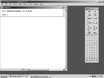
Figure 11.1: A Mathematica notebook that shows an input and output cell.

Mathematica commands are entered in a special syntax that corresponds closely to the way an expression is normally spoken. All function names start with an uppercase letter, and function arguments are enclosed in square brackets. For example, here is the Mathematica command for evaluating the definite integral of sin(x) from 0 to π:

    In[1]:= Integrate[Sin[x], {x, 0, Pi}]    Out[1]=  2

The terms Integrate and Sin are Mathematica functions. There are over two thousand built-in functions for performing a wide variety of calculations in fields such as algebra, calculus, statistics, number theory, and graphics.

Note

All examples of Mathematica commands are shown in a bold font to simulate how these commands look in a Mathematica notebook.

Mathematica Syntax

There is a close correspondence between MathML and the syntax used internally by Mathematica to represent mathematical formulas. The Mathematica syntax is, in effect, a text-based markup language for representing mathematical formulas and capturing both their notation and meaning. Because it provides a flexible and powerful system for describing mathematics, Mathematica was an important influence in the design of MathML. There are many points of similarity between the structure of MathML and the syntax of Mathematica expressions. In this section, we briefly review some details of Mathematica syntax and see how it compares with MathML.

Like MathML, Mathematica makes a distinction between the semantic meaning of a mathematical formula and its visual structure. The semantic meaning of any formula is represented internally using what is called its full form. This is a symbolic expression built up from standard Mathematica function names. The full form of a formula is closely analogous to MathML content markup. The appearance of mathematical notation, on the other hand, is described using a series of box structures, which are analogous to MathML presentation markup. Mathematica can freely convert between full-form expressions and boxes, using the former for performing computations and the latter for displaying mathematics in a notebook.

FullForm and Content MathML

The underlying logical structure of any mathematical formula, which determines its semantic interpretation, is called its full form. You can see the full form, of any expression expr by evaluating the command FullForm[expr]. For example, the following command shows the full form of the expression x² + y:

    In[1]:= FullForm[x^2+y]    Out[2]//FullForm= Plus[Power[x, 2], y]

The //FullForm annotation is added to the Out label to indicate that the output is being displayed in FullForm.

The content markup representation for the same expression would be as follows:

    <apply>    <plus/>    <apply>     <power/><ci>x</ci> <cn>2</cn>    </apply><ci>y</ci>    </apply>

You can see that the Mathematica full form of an expression and its content markup representation are very similar. Both use prefix functional notation to recursively build up complicated expressions out of smaller building blocks. The main difference is that in Mathematica, function application is indicated as f[x], where f is a specific Mathematica command such as Plus, Power, Sin, or Integrate. In content MathML, on the other hand, function application is indicated as <apply> f x </apply>, where f is a content markup element that represents a specific operator or function, such as plus, power, sin, or int. Also, the atomic units of mathematical notation (numbers, operators, and identifiers) are all denoted by a separate element in MathML, while Mathematica does not make any distinction between these different types of objects, encoding them all as strings.

Boxes and Presentation MathML

To describe the two-dimensional appearance of mathematical notation, Mathematica uses a series of box structures. There are different types of boxes for describing subscripts, superscripts, or fractions. Each of these box structures is in the form of a symbolic expression that can take one or more arguments. For example, the formula x² + y is represented in Mathematica by the following symbolic expression:

    RowBox[{SuperscriptBox["x", "2"], "+", "y"}]

There is a close correspondence between the box structures used in Mathematica and the presentation elements of MathML. For example, the above expression would be represented in presentation markup as shown below:

    <mrow>     <msup><mi>x</mi><mn>2</mn></msup>     <mo>+</mo><mi>y</mi>    </mrow>

You can see that the RowBox[…] and SuperscriptBox[…] constructs in Mathematica are equivalent to the <mrow>…</mrow> and <msup>…</msup> constructs in MathML. In each case, the child elements of the MathML presentation element are equivalent to the arguments of the Mathematica box expression. In the box expressions, as with full form, numbers, operators, and identifiers are all represented as strings.

A more complete listing of some Mathematica notational structures and their MathML counterparts is given in Table 11.1. The different types of boxes can be nested and combined, as necessary, to represent more complicated expressions.

Table 11.1: *Mathematica* Notational Structures and Their MathML Counterparts
Mathematica	MathML	Notation
`RowBox[x, y]`	`<mrow>…</mrow>`	x y
`FractionBox[x, y]`	`<mfrac>…</mfrac>`
`SqrtBox[x]`	`<msqrt>…</msqrt>`
`RadicalBox[x, y]`	`<mroot>…</mroot>`
`SubscriptBox[x, y]`	`<msub>…</msub>`	x_y
`SuperscriptBox[x, y]`	`<msup>…</msup>`	x^y
`SubsupercriptBox[x, y,z]`	`<msubsup>…</msubsup>`	x^z_y
`UnderscriptBox[x, y]`	`<munder>…</munder>`	x_y
`OverscriptBox[x, y]`	`<mover>…</mover>`	x^y
`UnderoverscriptBox[x, y,z]`	`<munderover>…</munderover>`	x^z_y
`GridBox[{x, y}]`	`<mtable>…</mtable>`	(x y)

You can see the underlying structure of any mathematical formula in a notebook by selecting the expression and choosing Format ▸ Show Expression from the menu. Figure 11.2 shows a formula in a notebook. Figure 11.3 shows the underlying expression for the formula.

click to expand
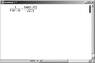
Figure 11.2: A mathematical formula in a notebook.

click to expand
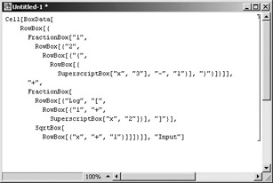
Figure 11.3: The underlying box structure of the formula shown in Figure 11.2 as displayed by using the Format ▸ Show Expression command.

Display Forms

Mathematica supports several different forms for the display of mathematics. A given formula can have several different textual representations, each corresponding to a different way of displaying the expression in a notebook. Some of the important display forms are:

InputForm: is a linear text-based form that can be typed directly using only the characters on a standard keyboard.
TraditionalForm: can display special characters and two-dimensional positioning to closely approximate traditional mathematical notation. It is not well-suited for computation since its mathematical meaning can be ambiguous.
StandardForm: is a compromise between InputForm and TraditionalForm. It can display special characters and two-dimensional layout while still preserving an unambiguous mathematical meaning. By default, input and output in Mathematica notebooks are displayed in StandardForm.
MathMLForm: displays the MathML markup for a mathematical expression. The markup is indented and formatted to reveal the hierarchical structure of the MathML expression.

Several other display forms (such as TeXForm and CForm) use the syntax of TeX and the C programming language, respectively. Forms that display expressions as a linear sequence of characters, such as FullForm and InputForm, are represented in Mathematica as simple strings. Forms that display two-dimensional notation, such as StandardForm and TraditionalForm, are represented using the box structures described earlier in this chapter.

To see an expression, expr, displayed in a particular form, you can type and evaluate the command form[expr]. Here are some examples of the same expression displayed in several different forms.

In StandardForm, the text is in a monospaced font, and square brackets are used for function application:

    In[1]:= StandardForm[x^2+1/Log[x]]

In TraditionalForm, variables are shown in italics, and parentheses are used for function application:

    In[2]:= TraditionalForm[x^2+1/Log[x]]

InputForm does not support two-dimensional display, so information about fractions and powers, for example, is shown in a linear syntax:

    In[3]:= InputForm[x^2+1/Log[x]]    Out[3]//InputForm= x^2 + Log[x]^(-1)

You can also convert a formula from one display form to another by selecting the formula and choosing the appropriate form in the Cell ▸ Convert To menu (Figure 11.4).

click to expand
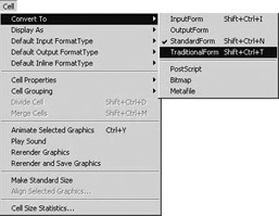
Figure 11.4: The Cell ▸ Convert To menu for changing between different display formats.

Figure 11.5 shows a notebook that contains an integral. Both the input and output are in StandardForm by default. ArcSin and Zeta are built-in Mathematica commands that represent the inverse sine and Riemann zeta functions, respectively.

click to expand
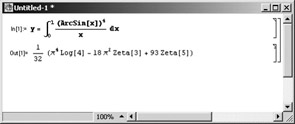
Figure 11.5: A mathematical formula, displayed in StandardForm, in a notebook. .

Figure 11.6 shows the same input and output cells from Figure 11.5 after they are converted to TraditionalForm using the Cell ▸ Convert To ▸ TraditionalForm menu. Notice that the ArcSin and Zeta functions are automatically displayed in the traditional notation for these functions.

click to expand
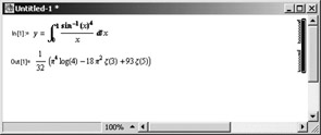
Figure 11.6: The same formula as in Figure 11.5 after conversion to TraditionalForm.

There are also several functions for converting between full form expressions and the various display forms (based on strings and boxes):

ToString[expr, form]: creates a string that represents the specified textual form of expr
ToBoxes[expr, form]: creates boxes that represent the specified textual form of expr
ToExpression[input, form]: creates an expression by interpreting a string or boxes as input in the specified textual form

The aim of this section is to provide an overview of the syntax used in Mathematica for representing the meaning and appearance of mathematical notation. If you want more details about the different types of expressions and display forms, you should consult the Mathematica documentation.

Exporting MathML from Mathematica

The next sections discusses menu commands in Mathematica.

Menu Commands

You can use Mathematica's typesetting capabilities to create nice-looking equations in a notebook, and then convert them into MathML for display on the Web. There are several ways to export mathematical expressions from a notebook as MathML.

To export a specific expression as MathML, select the expression and then choose the Edit ▸ Copy As ▸ MathML menu command. This copies the selected expression into the clipboard in the form of MathML presentation markup. You can then paste the markup into another application.

You can also export an entire notebook as HTML with MathML included. To do this, open the notebook and choose the File ▸ Save As Special ▸ XML (XHTML+MathML) menu command. This produces a well-formed and valid XHTML version of the notebook, with all mathematical formulas in the notebook automatically converted into MathML. The resulting document can then be displayed in any suitably configured Web browser, including Mozilla or IE with MathPlayer. Note that you should save the file with a .xml extension, for it to be viewable in the widest range of browsers.

Mathematica automatically inserts a reference to the Universal MathML stylesheet into the XHTML+MathML document. A local copy of this stylesheet is placed in a folder called HTMLFiles in the same directory as the XHTML+MathML file. This overcomes the limitation of IE not being able to use XSLT stylesheets from a remote location (see Section 7.2 for details on the Universal MathML stylesheet).

The Export Function

You can also export MathML to an external file using the built-in Mathematica function Export. This function takes various conversion options that you can use to customize the type of MathML generated. For example, you can choose to generate either presentation or content markup, add an XML declaration and a DOCTYPE declaration to the file, or add a specific namespace prefix to all the element and attribute names.

This function has the following syntax:

    Export[file, expr, format]

The first argument specifies the name of the file to which the data should be exported. The second argument specifies the data to be exported, and the third specifies the export format. Export is a versatile function that can be used to export text, graphics, typeset equations, and other content from Mathematica in a variety of formats. If you specify the export format as "MathML", the resulting output is in the form of MathML. Here is an example:

    In[3]:=  Export["test.mml", x^2+y, "MathML"]    Out[3]= test.mml

When you evaluate this command, Mathematica places the MathML representation of the expression x² + y into a file called test.mml. You can examine the contents of this file by evaluating the !!test.mml command. This prints the contents of the specified file in the notebook, giving the output shown below:

    In[4]:= !!test.mml    Out[4]= <math xmlns='http://www.w3.org/1998/Math/MathML'>    <semantics>     <mrow>      <msup>       <mi>x</mi>       <mn>2</mn>      </msup>      <mo>+</mo>      <mi>y</mi>     </mrow>     <annotation-xml encoding='MathML-Content'>      <apply>       <plus/>       <apply>        <power/>        <ci>x</ci>        <cn type='integer'>2</cn>       </apply>       <ci>y</ci>      </apply>      </annotation-xml>     </semantics>     </math>

By default, the file contains both presentation markup and content markup for the expression, which is enclosed in a semantics element. The xmlns attribute is added to the top-level math element to provide information about the namespace of the enclosed elements.

The ExportString Function

Another useful built-in function is ExportString. This works in the same way as Export except that it returns output in the form of a string instead of writing to an external file. This behavior is useful if you want to translate a Mathematica expression into MathML and get the output in the same notebook for subsequent manipulation. This function has the following syntax:

    ExportString[ expr, format]

Here is an example:

    In[5]:= ExportString[x+1,"MathML"]    Out[5]= <math xmlns='http://www.w3.org/1998/Math/MathML'>    <semantics>     <mrow>      <mi>x</mi>      <mo>+</mo>      <mn>1</mn>     </mrow>     <annotation-xml encoding='MathML-Content'>      <apply>       <plus/>       <ci>x</ci>        <cn type='integer'>1</cn>       </apply>      </annotation-xml>     </semantics>     <dis2> </math>

Export Conversion Options

You can modify the default behavior of the Export and ExportString functions by explicitly specifying one or more conversion options. The syntax for specifying a conversion option is given below:

     Export[file, expr, format, ConversionOptions ->         {option -> value}]    ExportString[ expr, format, ConversionOptions ->          <dis2> {option -> value}]

The following five conversion options are especially useful for exporting MathML:

"Formats": specifies the type of MathML generated. It is specified as a list whose elements can be "PresentationMathML" for presentation markup, and "ContentMathML" for content markup. The default value of this option is {"PresentationMathML", "ContentMathML"}, which generates combined parallel markup.
"NamespacePrefixes": specifies a namespace prefix that should be added to each element and attribute name in the generated MathML. It is specified in the form { url -> value}, where url is the URL associated with the namespace and value is the namespace prefix.
"Annotations": specifies whether an XML declaration or a DTD declaration should be added before the exported MathML expression. The option is specified as a list whose elements can be "DocumentHeader", "XMLDeclaration", and/or "DOCTYPEDeclaration". "DocumentHeader" is an overall switch that determines whether the other two values should take effect or not.
"Entities": specifies whether character entities are written out using names or numeric codes. The possible settings are "XML", "HTML", and "MathML". Each setting defines a set of named characters that are written out with their full names instead of the corresponding character codes.
"ElementFormatting": specifies the formatting of the MathML markup. If this option is set to "All", special indentation and linebreaking is used to indicate the tree structure of the markup. With a setting of "None", no special formatting is used.

Le's look at some examples of using these conversion options to control the form of the MathML generated.

The following command uses the "Formats" option to generate pure presentation markup:

    In[6]:= ExportString[x^2+y, "MathML",           ConversionOptions->{"Formats"->          {"PresentationMathML"}}]           Out[6]= <math xmlns='http://www.w3.org/1998/Math/MathML'>            <mrow>             <msup>              <mi>x</mi>              <mn>2</mn>             </msup>             <mo>+</mo>             <mi>y</mi>            </mrow>            </math>

The following command generates pure content markup, and uses conversion options to add the namespace prefix mml to each element and attribute name and to add a declaration for the MathML DTD at the start of the exported expression:

    In[7]:= ExportString[x^2+y,"MathML",           ConversionOptions->{"Formats"->{"ContentMathML"},           "Annotations"->{"DocumentHeader",           "DOCTYPEDeclaration"}, "NamespacePrefixes"->           http://www.w3.org/1998/Math/MathML"->"mml"}}]    Out[7]= <!DOCTYPE math PUBLIC '-//W3C//DTD MathML 2.0//EN'\          'http://www.w3.org/TR/MathML2/dtd/mathml2.dtd'>          <mml:math          xmlns:mml='http://www.w3.org/1998/Math/MathML'          xmlns='http://www.w3.org/1998/Math/MathML'>           <mml:apply>            <mml:plus/>            <mml:apply>             <mml:power/>              <mml:ci>x</mml:ci>              <mml:cn mml:type='integer'>2</mml:cn>             </mml:apply>             <mml:ci>y</mml:ci>            </mml:apply>            </mml:math>

By default, whenever Mathematica produces any MathML as output, character entities are specified using their Unicode values. This is to make the output readable in Web browsers, such as IE, that do not recognize MathML entity names.

Here is an example:

    In[8]:= ExportString[x*Sin[x],"MathML",           ConversionOptions->{"Formats"->           {"PresentationMathML"}}]    Out[8]:= "<math xmlns='http://www.w3.org/1998/Math/MathML'>                <mrow>                  <mi>&#945;</mi>                  <mo>&#8290;</mo>                  <mrow>                    <mi>sin</mi>                      <mo>&#8289;</mo>                      <mo>(</mo>                      <mi>x</mi>                      <mo>)</mo>                    </mrow>                  </mrow>                </math>"

However, by setting the conversion option, "Entities"->"MathML", you can tell Mathematica to write out the named entities instead., as shown here:

    In[8]:= ExportString[x*Sin[x],"MathML",           ConversionOptions->{"Formats"->           {"PresentationMathML"}, "Entities"->"MathML"}]    Out[8]:= "<math xmlns='http://www.w3.org/1998/Math/MathML'>                <mrow>                  <mi>&alpha;</mi>                  <mo>&InvisibleTimes;</mo>                  <mrow>                    <mi>sin</mi>                    <mo>&ApplyFunction;</mo>                    <mo>(</mo>                    <mi>x</mi>                    <mo>)</mo>                    </mrow>                  </mrow>                </math>"

All the above examples automatically apply indentation and linebreaking to the MathML output, so it is nicely formatted to display its tree structure. This behavior is controlled by the conversion option "ElementFormatting", whose default value is "All". If you prefer to get the MathML output without any extra formatting, you can set this option to "None". This produces more compact output, which is useful when you are exchanging data for machine processing, where the visual formatting is not important. Here is an example:

    In[8]:= ExportString[x*Sin[x],"MathML",           ConversionOptions->{"Formats"->           {"PresentationMathML"},"ElementFormatting"->"None"}]    In[8]:= "<math xmlns='http://www.w3.org/1998/Math/MathML'><mrow>    <mi>x</mi><mo>&#8290;</mo><mrow><mi>sin</mi><mo>&#8289;    </mo><mo>(</mo><mi>x</mi><mo>)</mo></mrow></mrow></math>"

For more details about the available conversion options and their allowed values, you should consult the product documentation.

Importing MathML into Mathematica

There are two ways to import MathML equations into Mathematica. The first way is to copy and paste MathML equations from another application directly into a notebook. When you paste a valid MathML expression into a notebook, Mathematica brings up a dialog that asks if you want to paste the literal markup or interpret it (Figure 11.7). If you choose to interpret the markup, it is automatically converted into Mathematica syntax.

click to expand
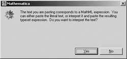
Figure 11.7: This dialog appears when you paste MathML markup into a Mathematica notebook.

Another way to import MathML expressions into a notebook is by evaluating the built-in Mathematica function, Import. This function has the following syntax:

    Import[file]    Import[file, format]

The first argument specifies the name of the file from which the data should be imported. Mathematica can use the file extension to identify the type of data in the file and to treat it accordingly. For example, any file with a .mml extension is automatically recognized as a MathML file and is converted into a Mathematica box expression. You can use the optional second argument to specify the export format explicitly. For importing MathML, the relevant import format is "MathML".

The following command creates a file called test.mml that contains the MathML markup corresponding to the expression, x∘2:

    In[1]:= Export["test.mml", x^2, "MathML"]    Out[1]= test.mml

The file test.mml contains the following MathML expression:

    <math xmlns='http://www.w3.org/1998/Math/MathML'>     <semantics>       <msup>         <mi>x</mi>         <mn>2</mn>       </msup>      <annotation-xml encoding='MathML-Content'>         <apply>           <power/>           <ci>x</ci>           <cn type='integer'>2</cn>         </apply>       </annotation-xml>      </semantics>    </math>

However, when the file is imported back into Mathematica, the MathML is automatically converted into a symbolic expression consisting of boxes, as shown here:

    In[2]:= Import["test.mml"]    Out[2]= FormBox[TagBox[TagBox[SuperscriptBox["x", "2"],            "MathMLPresentationTag", AutoDelete -> True],            "AnnotationsTagWrapper"[TagBox[SuperscriptBox[                 "x", "2"],            "MathMLContentTag", AutoDelete -> True]], AutoDelete ->            True], TraditionalForm]

The output of the last example is the Mathematica equivalent of the MathML expression. It contains information about both the appearance and meaning of the expression that was imported. You can convert this box expression into a mathematical expression using the function ToExpression, as shown here:

    In[3]:= ToExpression[%]    Out[3]= x²

MathML Conversion Functions

Mathematica 4.2 contains several functions for converting between MathML and the boxes and expressions used internally to represent mathematical formulas. Some of the important MathML functions are listed in Table 11.2.

Table 11.2: Important MathML Functions
Function	Description
`MathMLToExpression`	Converts a MathML string to a Mathematica expression
`ExpressionToMathML`	Converts a Mathematica expression to a MathML string
`MathMLToBoxes`	Converts a MathML string to a box expression
`BoxesToMathML`	Converts a box expression into MathML

These functions are all found in the context XML`MathML`. Hence, to evaluate any of these functions, you must add this context name as a prefix to the name of the function. Here is an example that shows how these functions work:

    In[1]:= XML`MathML`ExpressionToMathML[x^2]    Out[1] = <math xmlns='http://www.w3.org/1998/Math/MathML'>               <semantics>                <msup>                  <mi>x</mi>                  <mn>2</mn>                </msup>                <annotation-xml encoding='MathML-Content'>                  <apply>                    <power/>                    <ci>x</ci>                    <cn type='integer'>2</cn>                  </apply>                </annotation-xml>              </semantics>             </math>

You can specify any of the export conversion options listed earlier in this chapter directly in the functions that produce MathML. For example, the function XML `MathML `ExpressionToMathML yields both presentation and content markup enclosed in a semantics tag. But you can get either presentation or content markup alone by specifying the "Formats" conversion option. Here is an example:

    In[2]:= XML`MathML`ExpressionToMathML[x+1,"Formats"->           "PresentationMathML"]    Out[2]= <math xmlns='http://www.w3.org/1998/Math/MathML'>               <msup>                <mi>x</mi>                <mn>2</mn>               </msup>               </math>

You can add a namespace prefix to the output using the option "NamespacePrefixes", as shown here:

    In[3]:= XML`MathML`ExpressionToMathML[x+1,"Formats"->           "ContentMathML""NamespacePrefixes"->           {"http://www.w3.org/1998/Math/MathML"->"mml"}]    Out[3] = <math xmlns='http://www.w3.org/1998/Math/MathML'>                <m:apply>                 <m:power/>                 <m:ci>x</m:ci>                 <m:cn m:type='integer'>2</m:cn>                </m:apply>               </math>

The % command represents the result of the last calculation that you did in the notebook. The following command converts the MathML string back to a Mathematica expression:

    In[4]:= XML`MathML`MathMLToExpression[%]    Out[4] = x²

The following command converts a Mathematica box expression into the corresponding presentation MathML:

    In[5]:= XML`MathML`BoxesToMathML[SuperscriptBox["x","2"]]    Out[5] = <math xmlns='http://www.w3.org/1998/Math/MathML'>               <msup>                 <mi>x</mi>                 <mn>2</mn>                 </msup>              </math>

You can transform the MathML back into a box expression as shown here:

    In[3]:= XML`MathML`MathMLToBoxes[%]    Out[3] = FormBox[TagBox[SuperscriptBox[x,2],              MathMLPresentationTag, AutoDelete->True],TraditionalForm]

These examples demonstrate how closely MathML support is integrated into Mathematica. You can seamlessly and automatically convert mathematical expressions from Mathematica's syntax to MathML and vice versa. This makes it easy to integrate Mathematica with other applications using MathML as the format for exchanging mathematical information. In Section 12.5, we shall see some specific examples of how Mathematica and MathML can be combined to do computations in a Web browser.

The functions outlined above, for importing, exporting, and transforming MathML, are a special case of the more general XML processing capabilities available in Mathematica 4.2. You can import any arbitrary XML documents into Mathematica and then transform them using SymbolicXML. This is a format for representing XML documents as Mathematica expressions while preserving their tree structure. The advantage of converting XML documents into SymbolicXML is that you can apply to XML data any of Mathematica's built-in functions for numerical, symbolic, and graphical computations as well as functional programming. The MathML conversion functions discussed in this chapter are all implemented internally using SymbolicXML. The combination of SymbolicXML and Mathematica programming provides a useful alternative to other techniques for manipulating XML documents, such as XSLT transformations or the SAX or DOM APIs used with a low-level programming language such as Java.

< Day Day Up >