Example
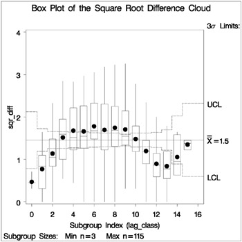
Example 80.1. A Box Plot of the Square Root Difference Cloud
The Gaussian form chosen for the variogram in the 'Getting Started' section on page 4852 is based on the consideration of the plots of the sample variogram. For the coal thickness data, the Gaussian form appears to be a reasonable choice.
It can often happen, however, that a plot of the sample variogram shows so much scatter that no particular form is evident. The cause of this scatter can be one or more outliers in the pairwise differences of the measured quantities .
A method of identifying potential outliers is discussed in Cressie (1993, section 2.2.2). This example illustrates how to use the OUTPAIR= data set from PROC VARIOGRAM to produce a square root difference cloud, which is useful in detecting outliers.
For the spatial process Z ( s ), s ˆˆ R 2 , the square root difference cloud for a particular direction e is given by
for a given lag distance h . In the actual computation, all pairs of points P 1 , P 2 within a distance tolerance around h and an angle tolerance around the direction e are used. This generates a number of point pairs for each lag class h . The spread of these values gives an indication of outliers.
Following the example in the 'Getting Started' section on page 4852, this example uses a basic lag distance of 7 units, with a distance tolerance of 3 . 5, and a direction of N_S, with a 30 o angle tolerance.
First, input the data, then use PROC VARIOGRAM to produce an OUTPAIR= data set. Then use a DATA step to subset this data by choosing pairs within 30 o of N_S. In addition, compute lag class and square root difference variables . Next, summarize the results using the MEANS procedure and present them in a box plot using the SHEWHART procedure. The box plot facilitates the detection of outliers.
You can conclude from this example that there does not appear to be any outliers in the N_S direction for the coal seam thickness data.
title 'Square Root Difference Cloud Example'; data thick; input east north thick @@; datalines; 0.7 59.6 34.1 2.1 82.7 42.2 4.7 75.1 39.5 4.8 52.8 34.3 5.9 67.1 37.0 6.0 35.7 35.9 6.4 33.7 36.4 7.0 46.7 34.6 8.2 40.1 35.4 13.3 0.6 44.7 13.3 68.2 37.8 13.4 31.3 37.8 17.8 6.9 43.9 20.1 66.3 37.7 22.7 87.6 42.8 23.0 93.9 43.6 24.3 73.0 39.3 24.8 15.1 42.3 24.8 26.3 39.7 26.4 58.0 36.9 26.9 65.0 37.8 27.7 83.3 41.8 27.9 90.8 43.3 29.1 47.9 36.7 29.5 89.4 43.0 30.1 6.1 43.6 30.8 12.1 42.8 32.7 40.2 37.5 34.8 8.1 43.3 35.3 32.0 38.8 37.0 70.3 39.2 38.2 77.9 40.7 38.9 23.3 40.5 39.4 82.5 41.4 43.0 4.7 43.3 43.7 7.6 43.1 46.4 84.1 41.5 46.7 10.6 42.6 49.9 22.1 40.7 51.0 88.8 42.0 52.8 68.9 39.3 52.9 32.7 39.2 55.5 92.9 42.2 56.0 1.6 42.7 60.6 75.2 40.1 62.1 26.6 40.1 63.0 12.7 41.8 69.0 75.6 40.1 70.5 83.7 40.9 70.9 11.0 41.7 71.5 29.5 39.8 78.1 45.5 38.7 78.2 9.1 41.7 78.4 20.0 40.8 80.5 55.9 38.7 81.1 51.0 38.6 83.8 7.9 41.6 84.5 11.0 41.5 85.2 67.3 39.4 85.5 73.0 39.8 86.7 70.4 39.6 87.2 55.7 38.8 88.1 0.0 41.6 88.4 12.1 41.3 88.4 99.6 41.2 88.8 82.9 40.5 88.9 6.2 41.5 90.6 7.0 41.5 90.7 49.6 38.9 91.5 55.4 39.0 92.9 46.8 39.1 93.4 70.9 39.7 94.8 71.5 39.7 96.2 84.3 40.3 98.2 58.2 39.5 proc variogram data=thick outp=outp; coordinates xc=east yc=north; var thick; compute novar; run; data sqroot; set outp; /*- Include only points +/- 30 degrees of N-S ------- */ where abs(cos) < .5; /*- Unit lag of 7, distance tolerance of 3.5 ------- */ lag_class=int(distance/7 + .5000001); sqr_diff=sqrt(abs(v1-v2)); run; proc sort data=sqroot; by lag_class; run; proc means data=sqroot noprint n mean std; var sqr_diff; by lag_class; output out=msqrt n=n mean=mean std=std; run; title2 'Summary of Results'; proc print data=msqrt; id lag_class; var n mean std; run; title 'Box Plot of the Square Root Difference Cloud'; proc shewhart data=sqroot; boxchart sqr_diff*lag_class / cframe=ligr haxis=axis1 vaxis=axis2; symbol1 v=dot c=blue height=3.5pct; axis1 minor=none; axis2 minor=none label=(angle=90 rotate=0); run;
| |
Square Root Difference Cloud Example Summary of Results lag_ class n mean std 0 5 0.47300 0.14263 1 31 0.77338 0.41467 2 55 1.13908 0.47604 3 58 1.51768 0.51989 4 63 1.67858 0.60494 5 61 1.66014 0.70687 6 75 1.77999 0.64590 7 85 1.69703 0.75362 8 84 1.74687 0.68785 9 115 1.70635 0.57173 10 82 1.48100 0.48105 11 85 1.19877 0.47121 12 68 0.89765 0.42510 13 38 0.84223 0.44249 14 7 1.05653 0.42548 15 3 1.35076 0.11472
| |
| |
| |
EAN: 2147483647
Pages: 132