Examples
| |
Example 19.1. Path Analysis: Stability of Alienation
The following covariance matrix from Wheaton, Muthen, Alwin, and Summers (1977) has served to illustrate the performance of several implementations for the analysis of structural equation models. Two different models have been analyzed by an early implementation of LISREL and are mentioned in J reskog (1978). You also can find a more detailed discussion of these models in the LISREL VI manual (J reskog and S rbom 1985). A slightly modified model for this covariance matrix is included in the EQS 2.0 manual (Bentler 1985, p. 28). The path diagram of this model is displayed in Figure 19.1. The same model is reanalyzed here by PROC CALIS. However, for the analysis with the EQS implementation, the last variable (V6) is rescaled by a factor of 0.1 to make the matrix less ill-conditioned. Since the Levenberg-Marquardt or Newton-Raphson optimization techniques are used with PROC CALIS, rescaling the data matrix is not necessary and, therefore, is not done here. The results reported here reflect the estimates based on the original covariance matrix.
data Wheaton(TYPE=COV); title "Stability of Alienation"; title2 "Data Matrix of WHEATON, MUTHEN, ALWIN & SUMMERS (1977)"; _type_ = 'cov'; input _name_ $ v1-v6; label v1='Anomia (1967)' v2='Anomia (1971)' v3='Education' v4='Powerlessness (1967)' v5='Powerlessness (1971)' v6='Occupational Status Index'; datalines; v1 11.834 . . . . . v2 6.947 9.364 . . . . v3 6.819 5.091 12.532 . . . v4 4.783 5.028 7.495 9.986 . . v5 -3.839 -3.889 -3.841 -3.625 9.610 . v6 -21.899 -18.831 -21.748 -18.775 35.522 450.288 ; proc calis cov data=Wheaton tech=nr edf=931 pall; Lineqs V1 = F1 + E1, V2 = .833 F1 + E2, V3 = F2 + E3, V4 = .833 F2 + E4, V5 = F3 + E5, V6 = Lamb (.5) F3 + E6, F1 = Gam1(-.5) F3 + D1, F2 = Beta (.5) F1 + Gam2(-.5) F3 + D2; Std E1-E6 = The1-The2 The1-The4 (6 * 3.), D1-D2 = Psi1-Psi2 (2 * 4.), F3 = Phi (6.) ; Cov E1 E3 = The5 (.2), E4 E2 = The5 (.2); run;
The COV option in the PROC CALIS statement requests the analysis of the covariance matrix. Without the COV option, the correlation matrix would be computed and analyzed. Since no METHOD= option has been used, maximum likelihood estimates are computed by default. The TECH=NR option requests the Newton-Raphson optimization method. The PALL option produces the almost complete set of displayed output, as displayed in Output 19.1.1 through Output 19.1.11. Note that, when you specify the PALL option, you can produce large amounts of output. The PALL option is used in this example to show how you can get a wide spectrum of useful information from PROC CALIS.
| |
Stability of Alienation Data Matrix of WHEATON, MUTHEN, ALWIN & SUMMERS (1977) The CALIS Procedure Covariance Structure Analysis: Pattern and Initial Values LINEQS Model Statement Matrix Rows Columns ------Matrix Type------ Term 1 1 _SEL_ 6 17 SELECTION 2 _BETA_ 17 17 EQSBETA IMINUSINV 3 _GAMMA_ 17 9 EQSGAMMA 4 _PHI_ 9 9 SYMMETRIC The 8 Endogenous Variables Manifest v1 v2 v3 v4 v5 v6 Latent F1 F2 The 9 Exogenous Variables Manifest Latent F3 Error E1 E2 E3 E4 E5 E6 D1 D2 Stability of Alienation Data Matrix of WHEATON, MUTHEN, ALWIN & SUMMERS (1977) Covariance Structure Analysis: Pattern and Initial Values v1 = 1.0000 F1 + 1.0000 E1 v2 = 0.8330 F1 + 1.0000 E2 v3 = 1.0000 F2 + 1.0000 E3 v4 = 0.8330 F2 + 1.0000 E4 v5 = 1.0000 F3 + 1.0000 E5 v6 = 0.5000*F3 + 1.0000 E6 Lamb Stability of Alienation Data Matrix of WHEATON, MUTHEN, ALWIN & SUMMERS (1977) Covariance Structure Analysis: Pattern and Initial Values F1 = -0.5000*F3 + 1.0000 D1 Gam1 F2 = 0.5000*F1 + -0.5000*F3 + 1.0000 D2 Beta Gam2 Stability of Alienation Data Matrix of WHEATON, MUTHEN, ALWIN & SUMMERS (1977) Covariance Structure Analysis: Pattern and Initial Values Variances of Exogenous Variables Variable Parameter Estimate F3 Phi 6.00000 E1 The1 3.00000 E2 The2 3.00000 E3 The1 3.00000 E4 The2 3.00000 E5 The3 3.00000 E6 The4 3.00000 D1 Psi1 4.00000 D2 Psi2 4.00000 Covariances Among Exogenous Variables Var1 Var2 Parameter Estimate E1 E3 The5 0.20000 E2 E4 The5 0.20000
| |
| |
Stability of Alienation Data Matrix of WHEATON, MUTHEN, ALWIN & SUMMERS (1977) Covariance Structure Analysis: Maximum Likelihood Estimation Observations 932 Model Terms 1 Variables 6 Model Matrices 4 Informations 21 Parameters 12 Variable Mean Std Dev v1 Anomia (1967) 0 3.44006 v2 Anomia (1971) 0 3.06007 v3 Education 0 3.54006 v4 Powerlessness (1967) 0 3.16006 v5 Powerlessness (1971) 0 3.10000 v6 Occupational Status Index 0 21.21999 Stability of Alienation Data Matrix of WHEATON, MUTHEN, ALWIN & SUMMERS (1977) Covariance Structure Analysis: Maximum Likelihood Estimation Covariances v1 v2 v3 v4 v5 v6 v1 Anomia (1967) 11.83400000 6.94700000 6.81900000 4.78300000 -3.83900000 -21.8990000 v2 Anomia (1971) 6.94700000 9.36400000 5.09100000 5.02800000 -3.88900000 -18.8310000 v3 Education 6.81900000 5.09100000 12.53200000 7.49500000 -3.84100000 -21.7480000 v4 Powerlessness (1967) 4.78300000 5.02800000 7.49500000 9.98600000 -3.62500000 -18.7750000 v5 Powerlessness (1971) -3.83900000 -3.88900000 -3.84100000 -3.62500000 9.61000000 35.5220000 v6 Occupational Status Index -21.89900000 -18.83100000 -21.74800000 -18.77500000 35.52200000 450.2880000 Determinant 6080570 Ln 15.620609 Stability of Alienation Data Matrix of WHEATON, MUTHEN, ALWIN & SUMMERS (1977) Covariance Structure Analysis: Maximum Likelihood Estimation Vector of Initial Estimates Parameter Estimate Type 1 Beta 0.50000 Matrix Entry: _BETA_[8:7] 2 Lamb 0.50000 Matrix Entry: _GAMMA_[6:1] 3 Gam1 -0.50000 Matrix Entry: _GAMMA_[7:1] 4 Gam2 -0.50000 Matrix Entry: _GAMMA_[8:1] 5 Phi 6.00000 Matrix Entry: _PHI_[1:1] 6 The1 3.00000 Matrix Entry: _PHI_[2:2] _PHI_[4:4] 7 The2 3.00000 Matrix Entry: _PHI_[3:3] _PHI_[5:5] 8 The5 0.20000 Matrix Entry: _PHI_[4:2] _PHI_[5:3] 9 The3 3.00000 Matrix Entry: _PHI_[6:6] 10 The4 3.00000 Matrix Entry: _PHI_[7:7] 11 Psi1 4.00000 Matrix Entry: _PHI_[8:8] 12 Psi2 4.00000 Matrix Entry: _PHI_[9:9]
| |
| |
Stability of Alienation Data Matrix of WHEATON, MUTHEN, ALWIN & SUMMERS (1977) Covariance Structure Analysis: Maximum Likelihood Estimation Predetermined Elements of the Predicted Moment Matrix v1 v2 v3 v4 v5 v6 v1 Anomia (1967) . . . . . . v2 Anomia (1971) . . . . . . v3 Education . . . . . . v4 Powerlessness (1967) . . . . . . v5 Powerlessness (1971) . . . . . . v6 Occupational Status Index . . . . . . Sum of Squared Differences 0
| |
| |
Stability of Alienation Data Matrix of WHEATON, MUTHEN, ALWIN & SUMMERS (1977) Covariance Structure Analysis: Maximum Likelihood Estimation Parameter Estimates 12 Functions (Observations) 21 Optimization Start Active Constraints 0 Objective Function 119.33282242 Max Abs Gradient Element 74.016932345 Ratio Between Actual Objective Max Abs and Function Active Objective Function Gradient Predicted Iter Restarts Calls Constraints Function Change Element Ridge Change 1 0 2 0 0.82689 118.5 1.3507 0 0.0154 2 0 3 0 0.09859 0.7283 0.2330 0 0.716 3 0 4 0 0.01581 0.0828 0.00684 0 1.285 4 0 5 0 0.01449 0.00132 0.000286 0 1.042 5 0 6 0 0.01448 9.936E-7 0.000045 0 1.053 6 0 7 0 0.01448 4.227E-9 1.685E-6 0 1.056 Optimization Results Iterations 6 Function Calls 8 Jacobian Calls 7 Active Constraints 0 Objective Function 0.0144844811 Max Abs Gradient Element 1.6847829E-6 Ridge 0 Actual Over Pred Change 1.0563204982 ABSGCONV convergence criterion satisfied.
| |
| |
Stability of Alienation Data Matrix of WHEATON, MUTHEN, ALWIN & SUMMERS (1977) Covariance Structure Analysis: Maximum Likelihood Estimation Predicted Model Matrix v1 v2 v3 v4 v5 v6 v1 Anomia (1967) 11.90390632 6.91059048 6.83016211 4.93499582 -4.16791157 -22.3768816 v2 Anomia (1971) 6.91059048 9.35145064 4.93499582 5.01664889 -3.47187034 -18.6399424 v3 Education 6.83016211 4.93499582 12.61574998 7.50355625 -4.06565606 -21.8278873 v4 Powerlessness (1967) 4.93499582 5.01664889 7.50355625 9.84539112 -3.38669150 -18.1826302 v5 Powerlessness (1971) -4.16791157 -3.47187034 -4.06565606 -3.38669150 9.61000000 35.5219999 v6 Occupational Status Index -22.37688158 -18.63994236 -21.82788734 -18.18263015 35.52199986 450.2879993 Determinant 6169285 Ln 15.635094 Stability of Alienation Data Matrix of WHEATON, MUTHEN, ALWIN & SUMMERS (1977) Covariance Structure Analysis: Maximum Likelihood Estimation Fit Function 0.0145 Goodness of Fit Index (GFI) 0.9953 GFI Adjusted for Degrees of Freedom (AGFI) 0.9890 Root Mean Square Residual (RMR) 0.2281 Parsimonious GFI (Mulaik, 1989) 0.5972 Chi-Square 13.4851 Chi-Square DF 9 Pr > Chi-Square 0.1419 Independence Model Chi-Square 2131.4 Independence Model Chi-Square DF 15 RMSEA Estimate 0.0231 RMSEA 90% Lower Confidence Limit . RMSEA 90% Upper Confidence Limit 0.0470 ECVI Estimate 0.0405 ECVI 90% Lower Confidence Limit . ECVI 90% Upper Confidence Limit 0.0556 Probability of Close Fit 0.9705 Bentler's Comparative Fit Index 0.9979 Normal Theory Reweighted LS Chi-Square 13.2804 Akaike's Information Criterion -4.5149 Bozdogan's (1987) CAIC -57.0509 Schwarz's Bayesian Criterion -48.0509 McDonald's (1989) Centrality 0.9976 Bentler & Bonett's (1980) Non-normed Index 0.9965 Bentler & Bonett's (1980) NFI 0.9937 James, Mulaik, & Brett (1982) Parsimonious NFI 0.5962 Z-Test of Wilson & Hilferty (1931) 1.0754 Bollen (1986) Normed Index Rho1 0.9895 Bollen (1988) Non-normed Index Delta2 0.9979 Hoelter's (1983) Critical N 1170
| |
| |
Stability of Alienation Data Matrix of WHEATON, MUTHEN, ALWIN & SUMMERS (1977) Covariance Structure Analysis: Maximum Likelihood Estimation Raw Residual Matrix v1 v2 v3 v4 v5 v6 v1 Anomia (1967) -.0699063150 0.0364095216 -.0111621061 -.1519958205 0.3289115712 0.4778815840 v2 Anomia (1971) 0.0364095216 0.0125493646 0.1560041795 0.0113511059 -.4171296612 -.1910576405 v3 Education -.0111621061 0.1560041795 -.0837499788 -.0085562504 0.2246560598 0.0798873380 v4 Powerlessness (1967) -.1519958205 0.0113511059 -.0085562504 0.1406088766 -.2383085022 -.5923698474 v5 Powerlessness (1971) 0.3289115712 -.4171296612 0.2246560598 -.2383085022 0.0000000000 0.0000000000 v6 Occupational Status Index 0.4778815840 -.1910576405 0.0798873380 -.5923698474 0.0000000000 0.0000000000 Average Absolute Residual 0.153928 Average Off-diagonal Absolute Residual 0.195045 Stability of Alienation Data Matrix of WHEATON, MUTHEN, ALWIN & SUMMERS (1977) Covariance Structure Analysis: Maximum Likelihood Estimation Rank Order of the 10 Largest Raw Residuals Row Column Residual v6 v4 -0.59237 v6 v1 0.47788 v5 v2 -0.41713 v5 v1 0.32891 v5 v4 -0.23831 v5 v3 0.22466 v6 v2 -0.19106 v3 v2 0.15600 v4 v1 -0.15200 v4 v4 0.14061 Stability of Alienation Data Matrix of WHEATON, MUTHEN, ALWIN & SUMMERS (1977) Covariance Structure Analysis: Maximum Likelihood Estimation Asymptotically Standardized Residual Matrix v1 v2 v3 v4 v5 v6 v1 Anomia (1967) -0.308548787 0.526654452 -0.056188826 -0.865070455 2.553366366 0.464866661 v2 Anomia (1971) 0.526654452 0.054363484 0.876120855 0.057354415 -2.763708659 -0.170127806 v3 Education -0.056188826 0.876120855 -0.354347092 -0.121874301 1.697931678 0.070202664 v4 Powerlessness (1967) -0.865070455 0.057354415 -0.121874301 0.584930625 -1.557412695 -0.495982427 v5 Powerlessness (1971) 2.553366366 -2.763708659 1.697931678 -1.557412695 0.000000000 0.000000000 v6 Occupational Status Index 0.464866661 -0.170127806 0.070202664 -0.495982427 0.000000000 0.000000000 Average Standardized Residual 0.646622 Average Off-diagonal Standardized Residual 0.818457 Stability of Alienation Data Matrix of WHEATON, MUTHEN, ALWIN & SUMMERS (1977) Covariance Structure Analysis: Maximum Likelihood Estimation Rank Order of the 10 Largest Asymptotically Standardized Residuals Row Column Residual v5 v2 -2.76371 v5 v1 2.55337 v5 v3 1.69793 v5 v4 -1.55741 v3 v2 0.87612 v4 v1 -0.86507 v4 v4 0.58493 v2 v1 0.52665 v6 v4 -0.49598 v6 v1 0.46487 Stability of Alienation Data Matrix of WHEATON, MUTHEN, ALWIN & SUMMERS (1977) Covariance Structure Analysis: Maximum Likelihood Estimation Distribution of Asymptotically Standardized Residuals Each * Represents 1 Residuals ----------Range--------- Freq Percent -3.00000 -2.75000 1 4.76 * -2.75000 -2.50000 0 0.00 -2.50000 -2.25000 0 0.00 -2.25000 -2.00000 0 0.00 -2.00000 -1.75000 0 0.00 -1.75000 -1.50000 1 4.76 * -1.50000 -1.25000 0 0.00 -1.25000 -1.00000 0 0.00 -1.00000 -0.75000 1 4.76 * -0.75000 -0.50000 0 0.00 -0.50000 -0.25000 3 14.29 *** -0.25000 0 3 14.29 *** 0 0.25000 6 28.57 ****** 0.25000 0.50000 1 4.76 * 0.50000 0.75000 2 9.52 ** 0.75000 1.00000 1 4.76 * 1.00000 1.25000 0 0.00 1.25000 1.50000 0 0.00 1.50000 1.75000 1 4.76 * 1.75000 2.00000 0 0.00 2.00000 2.25000 0 0.00 2.25000 2.50000 0 0.00 2.50000 2.75000 1 4.76 *
| |
| |
Stability of Alienation Data Matrix of WHEATON, MUTHEN, ALWIN & SUMMERS (1977) Covariance Structure Analysis: Maximum Likelihood Estimation v1 = 1.0000 F1 + 1.0000 E1 v2 = 0.8330 F1 + 1.0000 E2 v3 = 1.0000 F2 + 1.0000 E3 v4 = 0.8330 F2 + 1.0000 E4 v5 = 1.0000 F3 + 1.0000 E5 v6 = 5.3688*F3 + 1.0000 E6 Std Err 0.4337 Lamb t Value 12.3788 Stability of Alienation Data Matrix of WHEATON, MUTHEN, ALWIN & SUMMERS (1977) Covariance Structure Analysis: Maximum Likelihood Estimation F1 = -0.6299*F3 + 1.0000 D1 Std Err 0.0563 Gam1 t Value -11.1809 F2 = 0.5931*F1 + -0.2409*F3 + 1.0000 D2 Std Err 0.0468 Beta 0.0549 Gam2 t Value 12.6788 -4.3885 Stability of Alienation Data Matrix of WHEATON, MUTHEN, ALWIN & SUMMERS (1977) Covariance Structure Analysis: Maximum Likelihood Estimation Variances of Exogenous Variables Standard Variable Parameter Estimate Error t Value F3 Phi 6.61632 0.63914 10.35 E1 The1 3.60788 0.20092 17.96 E2 The2 3.59493 0.16448 21.86 E3 The1 3.60788 0.20092 17.96 E4 The2 3.59493 0.16448 21.86 E5 The3 2.99368 0.49861 6.00 E6 The4 259.57580 18.31150 14.18 D1 Psi1 5.67047 0.42301 13.41 D2 Psi2 4.51480 0.33532 13.46 Covariances Among Exogenous Variables Standard Var1 Var2 Parameter Estimate Error t Value E1 E3 The5 0.90580 0.12167 7.44 E2 E4 The5 0.90580 0.12167 7.44
| |
| |
Stability of Alienation Data Matrix of WHEATON, MUTHEN, ALWIN & SUMMERS (1977) Covariance Structure Analysis: Maximum Likelihood Estimation v1 = 0.8348 F1 + 0.5505 E1 v2 = 0.7846 F1 + 0.6200 E2 v3 = 0.8450 F2 + 0.5348 E3 v4 = 0.7968 F2 + 0.6043 E4 v5 = 0.8297 F3 + 0.5581 E5 v6 = 0.6508*F3 + 0.7593 E6 Lamb Stability of Alienation Data Matrix of WHEATON, MUTHEN, ALWIN & SUMMERS (1977) Covariance Structure Analysis: Maximum Likelihood Estimation F1 = -0.5626*F3 + 0.8268 D1 Gam1 F2 = 0.5692*F1 + -0.2064*F3 + 0.7080 D2 Beta Gam2 Stability of Alienation Data Matrix of WHEATON, MUTHEN, ALWIN & SUMMERS (1977) Covariance Structure Analysis: Maximum Likelihood Estimation Squared Multiple Correlations Error Total Variable Variance Variance R-Square 1 v1 3.60788 11.90391 0.6969 2 v2 3.59493 9.35145 0.6156 3 v3 3.60788 12.61575 0.7140 4 v4 3.59493 9.84539 0.6349 5 v5 2.99368 9.61000 0.6885 6 v6 259.57580 450.28800 0.4235 7 F1 5.67047 8.29603 0.3165 8 F2 4.51480 9.00787 0.4988 Correlations Among Exogenous Variables Var1 Var2 Parameter Estimate E1 E3 The5 0.25106 E2 E4 The5 0.25197 Stability of Alienation Data Matrix of WHEATON, MUTHEN, ALWIN & SUMMERS (1977) Covariance Structure Analysis: Maximum Likelihood Estimation Predicted Moments of Latent Variables F1 F2 F3 F1 8.296026985 5.924364730 -4.167911571 F2 5.924364730 9.007870649 -4.065656060 F3 -4.167911571 -4.065656060 6.616317547 Predicted Moments between Manifest and Latent Variables F1 F2 F3 v1 8.29602698 5.92436473 -4.16791157 v2 6.91059048 4.93499582 -3.47187034 v3 5.92436473 9.00787065 -4.06565606 v4 4.93499582 7.50355625 -3.38669150 v5 -4.16791157 -4.06565606 6.61631755 v6 -22.37688158 -21.82788734 35.52199986
| |
| |
Stability of Alienation Data Matrix of WHEATON, MUTHEN, ALWIN & SUMMERS (1977) Covariance Structure Analysis: Maximum Likelihood Estimation Latent Variable Score Regression Coefficients F1 F2 F3 v1 Anomia (1967) 0.4131113567 0.0482681051 -.0521264408 v2 Anomia (1971) 0.3454029627 0.0400143300 -.0435560637 v3 Education 0.0526632293 0.4306175653 -.0399927539 v4 Powerlessness (1967) 0.0437036855 0.3600452776 -.0334000265 v5 Powerlessness (1971) -.0749215200 -.0639697183 0.5057060770 v6 Occupational Status Index -.0046390513 -.0039609288 0.0313127184 Total Effects F3 F1 F2 v1 -0.629944307 1.000000000 0.000000000 v2 -0.524743608 0.833000000 0.000000000 v3 -0.614489258 0.593112208 1.000000000 v4 -0.511869552 0.494062469 0.833000000 v5 1.000000000 0.000000000 0.000000000 v6 5.368847492 0.000000000 0.000000000 F1 -0.629944307 0.000000000 0.000000000 F2 -0.614489258 0.593112208 0.000000000 Indirect Effects F3 F1 F2 v1 -.6299443069 0.0000000000 0 v2 -.5247436076 0.0000000000 0 v3 -.6144892580 0.5931122083 0 v4 -.5118695519 0.4940624695 0 v5 0.0000000000 0.0000000000 0 v6 0.0000000000 0.0000000000 0 F1 0.0000000000 0.0000000000 0 F2 -.3736276589 0.0000000000 0
| |
| |
Stability of Alienation Data Matrix of WHEATON, MUTHEN, ALWIN & SUMMERS (1977) Covariance Structure Analysis: Maximum Likelihood Estimation Lagrange Multiplier and Wald Test Indices _PHI_ [9:9] Symmetric Matrix Univariate Tests for Constant Constraints Lagrange Multiplier or Wald Index / Probability / Approx Change of Value F3 E1 E2 E3 E4 E5 E6 D1 D2 F3 107.1619 3.3903 3.3901 0.5752 0.5753 . . . . . 0.0656 0.0656 0.4482 0.4482 . . . . . 0.5079 -0.4231 0.2090 -0.1741 . . . . [Phi] Sing Sing Sing Sing E1 3.3903 322.4501 0.1529 55.4237 1.2037 5.8025 0.7398 0.4840 0.0000 0.0656 . 0.6958 . 0.2726 0.0160 0.3897 0.4866 0.9961 0.5079 . 0.0900 . -0.3262 0.5193 -1.2587 0.2276 0.0014 [The1] [The5] E2 3.3901 0.1529 477.6768 0.5946 55.4237 7.3649 1.4168 0.4840 0.0000 0.0656 0.6958 . 0.4406 . 0.0067 0.2339 0.4866 0.9961 -0.4231 0.0900 . 0.2328 . -0.5060 1.5431 -0.1896 -0.0011 [The2] [The5] E3 0.5752 55.4237 0.5946 322.4501 0.1528 1.5982 0.0991 1.1825 0.5942 0.4482 . 0.4406 . 0.6958 0.2062 0.7529 0.2768 0.4408 0.2090 . 0.2328 . -0.0900 0.2709 -0.4579 0.2984 -0.2806 [The5] [The1] E4 0.5753 1.2037 55.4237 0.1528 477.6768 1.2044 0.0029 1.1825 0.5942 0.4482 0.2726 . 0.6958 . 0.2724 0.9568 0.2768 0.4408 -0.1741 -0.3262 . -0.0900 . -0.2037 0.0700 -0.2486 0.2338 [The5] [The2] E5 . 5.8025 7.3649 1.5982 1.2044 36.0486 . 0.1033 0.1035 . 0.0160 0.0067 0.2062 0.2724 . . 0.7479 0.7477 . 0.5193 -0.5060 0.2709 -0.2037 . . -0.2776 0.1062 Sing [The3] Sing E6 . 0.7398 1.4168 0.0991 0.0029 . 200.9466 0.1034 0.1035 . 0.3897 0.2339 0.7529 0.9568 . . 0.7478 0.7477 . -1.2587 1.5431 -0.4579 0.0700 . . 1.4906 -0.5700 Sing Sing [The4] D1 . 0.4840 0.4840 1.1825 1.1825 0.1033 0.1034 179.6950 . . 0.4866 0.4866 0.2768 0.2768 0.7479 0.7478 . . . 0.2276 -0.1896 0.2984 -0.2486 -0.2776 1.4906 . . Sing [Psi1] Sing D2 . 0.0000 0.0000 0.5942 0.5942 0.1035 0.1035 . 181.2787 . 0.9961 0.9961 0.4408 0.4408 0.7477 0.7477 . . . 0.0014 -0.0011 -0.2806 0.2338 0.1062 -0.5700 . . Sing Sing [Psi2] Stability of Alienation Data Matrix of WHEATON, MUTHEN, ALWIN & SUMMERS (1977) Covariance Structure Analysis: Maximum Likelihood Estimation Rank Order of the 10 Largest Lagrange Multipliers in _PHI_ Row Column Chi-Square Pr > ChiSq E5 E2 7.36486 0.0067 E5 E1 5.80246 0.0160 E1 F3 3.39030 0.0656 E2 F3 3.39013 0.0656 E5 E3 1.59820 0.2062 E6 E2 1.41677 0.2339 E5 E4 1.20437 0.2724 E4 E1 1.20367 0.2726 D1 E3 1.18251 0.2768 D1 E4 1.18249 0.2768 Stability of Alienation Data Matrix of WHEATON, MUTHEN, ALWIN & SUMMERS (1977) Covariance Structure Analysis: Maximum Likelihood Estimation Lagrange Multiplier and Wald Test Indices _GAMMA_ [8:1] General Matrix Univariate Tests for Constant Constraints Lagrange Multiplier or Wald Index / Probability / Approx Change of Value F3 v1 3.3903 0.0656 0.0768 v2 3.3901 0.0656 -0.0639 v3 0.5752 0.4482 0.0316 v4 0.5753 0.4482 -0.0263 v5 . . . Sing v6 153.2354 . . [Lamb] F1 125.0132 . . [Gam1] F2 19.2585 . . [Gam2] Stability of Alienation Data Matrix of WHEATON, MUTHEN, ALWIN & SUMMERS (1977) Covariance Structure Analysis: Maximum Likelihood Estimation Rank Order of the 4 Largest Lagrange Multipliers in _GAMMA_ Row Column Chi-Square Pr > ChiSq v1 F3 3.39030 0.0656 v2 F3 3.39013 0.0656 v4 F3 0.57526 0.4482 v3 F3 0.57523 0.4482 Stability of Alienation Data Matrix of WHEATON, MUTHEN, ALWIN & SUMMERS (1977) Covariance Structure Analysis: Maximum Likelihood Estimation Lagrange Multiplier and Wald Test Indices _BETA_ [8:8] General Matrix Identity-Minus-Inverse Model Matrix Univariate Tests for Constant Constraints Lagrange Multiplier or Wald Index / Probability / Approx Change of Value v1 v2 v3 v4 v5 v6 F1 F2 v1 . 0.1647 0.0511 0.8029 5.4083 0.1233 0.4047 0.4750 . 0.6849 0.8212 0.3702 0.0200 0.7255 0.5247 0.4907 . -0.0159 -0.0063 -0.0284 0.0697 0.0015 -0.0257 -0.0239 Sing v2 0.5957 . 0.6406 0.0135 5.8858 0.0274 0.4047 0.4750 0.4402 . 0.4235 0.9076 0.0153 0.8686 0.5247 0.4907 0.0218 . 0.0185 0.0032 -0.0609 -0.0006 0.0214 0.0199 Sing v3 0.3839 0.3027 . 0.1446 1.1537 0.0296 0.1588 0.0817 0.5355 0.5822 . 0.7038 0.2828 0.8634 0.6902 0.7750 0.0178 0.0180 . -0.0145 0.0322 0.0007 0.0144 -0.0110 Sing v4 0.4487 0.2519 0.0002 . 0.9867 0.1442 0.1588 0.0817 0.5030 0.6157 0.9877 . 0.3206 0.7041 0.6903 0.7750 -0.0160 -0.0144 -0.0004 . -0.0249 -0.0014 -0.0120 0.0092 Sing v5 5.4085 8.6455 2.7123 2.1457 . . 0.1033 0.1035 0.0200 0.0033 0.0996 0.1430 . . 0.7479 0.7476 0.1242 -0.1454 0.0785 -0.0674 . . -0.0490 0.0329 Sing Sing v6 0.4209 1.4387 0.3044 0.0213 . . 0.1034 0.1035 0.5165 0.2304 0.5811 0.8841 . . 0.7478 0.7477 -0.2189 0.3924 -0.1602 0.0431 . . 0.2629 -0.1765 Sing Sing F1 1.0998 1.1021 1.6114 1.6128 0.1032 0.1035 . . 0.2943 0.2938 0.2043 0.2041 0.7480 0.7477 . . 0.0977 -0.0817 0.0993 -0.0831 -0.0927 0.0057 . . Sing Sing v F2 0.0193 0.0194 0.4765 0.4760 0.1034 0.1035 160.7520 . 0.8896 0.8892 0.4900 0.4902 0.7477 0.7477 . . -0.0104 0.0087 -0.0625 0.0522 0.0355 -0.0022 . . [Beta] Sing Stability of Alienation Data Matrix of WHEATON, MUTHEN, ALWIN & SUMMERS (1977) Covariance Structure Analysis: Maximum Likelihood Estimation Rank Order of the 10 Largest Lagrange Multipliers in _BETA_ Row Column Chi-Square Pr > ChiSq v5 v2 8.64546 0.0033 v2 v5 5.88576 0.0153 v5 v1 5.40848 0.0200 v1 v5 5.40832 0.0200 v5 v3 2.71233 0.0996 v5 v4 2.14572 0.1430 F1 v4 1.61279 0.2041 F1 v3 1.61137 0.2043 v6 v2 1.43867 0.2304 v3 v5 1.15372 0.2828
| |
| |
Stability of Alienation Data Matrix of WHEATON, MUTHEN, ALWIN & SUMMERS (1977) Covariance Structure Analysis: Maximum Likelihood Estimation Univariate Lagrange Multiplier Test for Releasing Equality Constraints Equality Constraint -----Changes----- Chi-Square Pr > ChiSq [E1:E1] = [E3:E3] 0.0293 -0.0308 0.02106 0.8846 [E2:E2] = [E4:E4] -0.1342 0.1388 0.69488 0.4045 [E3:E1] = [E4:E2] 0.2468 -0.1710 1.29124 0.2558
| |
Output 19.1.1 displays the model specification in matrix terms, followed by the lists of endogenous and exogenous variables. Equations and initial parameter estimates are also displayed. You can use this information to ensure that the desired model is the model being analyzed.
General modeling information and simple descriptive statistics are displayed in Output 19.1.2. Because the input data set contains only the covariance matrix, the means of the manifest variables are assumed to be zero. Note that this has no impact on the estimation, unless a mean structure model is being analyzed. The twelve parameter estimates in the model and their respective locations in the parameter matrices are also displayed. Each of the parameters, The1 , The2 , and The5 , is specified for two elements in the parameter matrix _PHI_ .
PROC CALIS examines whether each element in the moment matrix is modeled by the parameters defined in the model. If an element is not structured by the model parameters, it is predetermined by its observed value. This occurs, for example, when there are exogenous manifest variables in the model. If present, the predetermined values of the elements will be displayed. In the current example, the ˜.' displayed for all elements in the predicted moment matrix (Output 19.1.3) indicates that there are no predetermined elements in the model.
Output 19.1.4 displays the optimization information. You can check this table to determine whether the convergence criterion is satisfied. PROC CALIS displays an error message when problematic solutions are encountered .
The predicted model matrix is displayed next , followed by a list of model test statistics or fit indices (Output 19.1.5). Depending on your modeling philosophy, some indices may be preferred to others. In this example, all indices and test statistics point to a good fit of the model.
PROC CALIS can perform a detailed residual analysis. Large residuals may indicate misspecification of the model. In Output 19.1.6 for example, note the table for the 10 largest asymptotically standardized residuals. As the table shows, the specified model performs the poorest concerning the variable V5 and its covariance with V2 , V1 , and V3 . This may be the result of a misspecification of the model equation for V5 . However, because the model fit is quite good, such a possible misspecification may have no practical significance and is not a serious concern in the analysis.
Output 19.1.7 displays the equations and parameter estimates. Each parameter estimate is displayed with its standard error and the corresponding t ratio. As a general rule, a t ratio larger than 2 represents a statistically significant departure from 0. From these results, it is observed that both F1 (Alienation 1967) and F2 (Alienation 1971) are regressed negatively on F3 (Socioeconomic Status), and F1 has a positive effect on F2 . The estimates and significance tests for the variance and covariance of the exogenous variables are also displayed.
The measurement scale of variables is often arbitrary. Therefore, it can be useful to look at the standardized equations produced by PROC CALIS. Output 19.1.8 displays the standardized equations and predicted moments. From the standardized structural equations for F1 and F2 , you can conclude that SES ( F3 ) has a larger impact on earlier Alienation ( F1 )thanonlaterAlienation( F3 ).
The squared multiple correlation for each equation, the correlation among the exogenous variables, and the covariance matrices among the latent variables and between the observed and the latent variables help to describe the relationships among all variables.
Output 19.1.9 displays the latent variable score regression coefficients that produce the latent variable scores. Each latent variable is expressed as a linear combination of the observed variables. See Chapter 64, 'The SCORE Procedure,' for more information on the creation of latent variable scores. Note that the total effects and indirect effects of the exogenous variables are also displayed.
PROC CALIS can display Lagrange multiplier and Wald statistics for model modifications. Modification indices are displayed for each parameter matrix. Only the Lagrange multiplier statistics have significance levels and approximate changes of values displayed. The significance level of the Wald statistic for a given parameter is the same as that shown in the equation output. An insignificant p -value for a Wald statistic means that the corresponding parameter can be dropped from the model without significantly worsening the fit of the model.
A significant p -value for a Lagrange multiplier test indicates that the model would achieve a better fit if the corresponding parameter is free. To aid in determining significant results, PROC CALIS displays the rank order of the ten largest Lagrange multiplier statistics. For example, [E5:E2] in the _PHI_ matrix is associated with the largest Lagrange multiplier statistic; the associated p -value is 0.0067. This means that adding a parameter for the covariance between E5 and E2 will lead to a significantly better fit of the model. However, adding parameters indiscriminately can result in specification errors. An over-fitted model may not perform well with future samples. As always, the decision to add parameters should be accompanied with consideration and knowledge of the application area.
When you specify equality constraints, PROC CALIS displays Lagrange multiplier tests for releasing the constraints. In the current example, none of the three constraints achieve a p -value smaller than 0.05. This means that releasing the constraints may not lead to a significantly better fit of the model. Therefore, all constraints are retained in the model.
The model is specified using the LINEQS, STD, and COV statements. The section 'Getting Started' on page 560 also contains the COSAN and RAM specifications of this model. These model specifications would give essentially the same results.
proc calis cov data=Wheaton tech=nr edf=931; Cosan J(9, Ide) * A(9, Gen, Imi) * P(9, Sym); Matrix A [ ,7] = 1. .833 5 * 0. Beta (.5) , [ ,8] = 2 * 0. 1. .833 , [ ,9] = 4 * 0. 1. Lamb Gam1-Gam2 (.5 2 * -.5); Matrix P [1,1] = The1-The2 The1-The4 (6 * 3.) , [7,7] = Psi1-Psi2 Phi (2 * 4. 6.) , [3,1] = The5 (.2) , [4,2] = The5 (.2) ; Vnames J V1-V6 F1-F3 , A = J , P E1-E6 D1-D3 ; run; proc calis cov data=Wheaton tech=nr edf=931; Ram 1 1 7 1. , 1 2 7 .833 , 1 3 8 1. , 1 4 8 .833 , 1 5 9 1. , 1 6 9 .5 Lamb , 1 7 9 -.5 Gam1 , 1 8 7 .5 Beta , 1 8 9 -.5 Gam2 , 2 1 1 3. The1 , 2 2 2 3. The2 , 2 3 3 3. The1 , 2 4 4 3. The2 , 2 5 5 3. The3 , 2 6 6 3. The4 , 2 1 3 .2 The5 , 2 2 4 .2 The5 , 2 7 7 4. Psi1 , 2 8 8 4. Psi2 , 2 9 9 6. Phi ; Vnames 1 F1-F3, 2 E1-E6 D1-D3; run;
Example 19.2. Simultaneous Equations with Intercept
The demand-and-supply food example of Kmenta (1971, pp. 565, 582) is used to illustrate the use of PROC CALIS for the estimation of intercepts and coefficients of simultaneous equations. The model is specified by two simultaneous equations containing two endogenous variables Q and P and three exogenous variables D , F , and Y ,
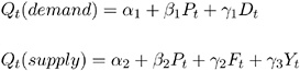
for t =1, , 20.
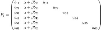
The LINEQS statement requires that each endogenous variable appear on the left-hand side of exactly one equation. Instead of analyzing the system
PROC CALIS analyzes the equivalent system
with B * = I ˆ’ B . This requires that one of the preceding equations be solved for P t . Solving the second equation for P t yields
You can estimate the intercepts of a system of simultaneous equations by applying PROC CALIS on the uncorrected covariance (UCOV) matrix of the data set that is augmented by an additional constant variable with the value 1. In the following example, the uncorrected covariance matrix is augmented by an additional variable INTERCEPT by using the AUGMENT option. The PROC CALIS statement contains the options UCOV and AUG to compute and analyze an augmented UCOV matrix from the input data set FOOD.
Data food; Title 'Food example of KMENTA(1971, p.565 & 582)'; Input Q P D F Y; Label Q='Food Consumption per Head' P='Ratio of Food Prices to General Price' D='Disposable Income in Constant Prices' F='Ratio of Preceding Years Prices' Y='Time in Years 1922-1941'; datalines; 98.485 100.323 87.4 98.0 1 99.187 104.264 97.6 99.1 2 102.163 103.435 96.7 99.1 3 101.504 104.506 98.2 98.1 4 104.240 98.001 99.8 110.8 5 103.243 99.456 100.5 108.2 6 103.993 101.066 103.2 105.6 7 99.900 104.763 107.8 109.8 8 100.350 96.446 96.6 108.7 9 102.820 91.228 88.9 100.6 10 95.435 93.085 75.1 81.0 11 92.424 98.801 76.9 68.6 12 94.535 102.908 84.6 70.9 13 98.757 98.756 90.6 81.4 14 105.797 95.119 103.1 102.3 15 100.225 98.451 105.1 105.0 16 103.522 86.498 96.4 110.5 17 99.929 104.016 104.4 92.5 18 105.223 105.769 110.7 89.3 19 106.232 113.490 127.1 93.0 20 ; proc calis ucov aug data=food pshort; Title2 'Compute ML Estimates With Intercept'; Lineqs Q = alf1 Intercept + alf2 P + alf3 D + E1, P = gam1 Intercept + gam2 Q + gam3 F + gam4 Y + E2; Std E1-E2 = eps1-eps2; Cov E1-E2 = eps3; Bounds eps1-eps2 >= 0. ; run;
The following, essentially equivalent model definition uses program code to reparameterize the model in terms of the original equations; the output is displayed in Output 19.2.1.
proc calis data=food ucov aug pshort; Lineqs Q = alphal Intercept + beta1 P + gamma1 D + E1, P = alpha2_b Intercept + gamma2_b F + gamma3_b Y + _b Q + E2; Std E1-E2 = eps1-eps2; Cov E1-E2 = eps3; Parameters alpha2 (50.) beta2 gamma2 gamma3 (3*.25); alpha2_b = -alpha2 / beta2; gamma2_b = -gamma2 / beta2; gamma3_b = -gamma3 / beta2; _b = 1 / beta2; Bounds eps1-eps2 >= 0. ; run;
| |
Food example of KMENTA(1971, p.565 & 582) The CALIS Procedure Covariance Structure Analysis: Pattern and Initial Values LINEQS Model Statement Matrix Rows Columns ------Matrix Type------- Term 1 1 _SEL_ 6 8 SELECTION 2 _BETA_ 8 8 EQSBETA IMINUSINV 3 _GAMMA_ 8 6 EQSGAMMA 4 _PHI_ 6 6 SYMMETRIC The 2 Endogenous Variables Manifest Q P Latent The 6 Exogenous Variables Manifest D F Y Intercept Latent Error E1 E2 Covariance Structure Analysis: Maximum Likelihood Estimation Parameter Estimates 10 Functions (Observations) 21 Lower Bounds 2 Upper Bounds 0 Optimization Start Active Constraints 0 Objective Function 2.350006504 Max Abs Gradient Element 203.97414363 Radius 62167.829154 Ratio Between Actual Objective Max Abs and Function Active Objective Function Gradient Predicted Iter Restarts Calls Constraints Function Change Element Lambda Change 1 0 2 0 1.19094 1.1591 3.9410 0 0.688 2 0 5 0 0.32678 0.8642 9.9864 0.00127 2.356 3 0 7 0 0.19108 0.1357 5.5100 0.00006 0.685 4 0 10 0 0.16682 0.0243 2.0513 0.00005 0.867 5 0 12 0 0.16288 0.00393 1.0570 0.00014 0.828 6 0 13 0 0.16132 0.00156 0.3643 0.00004 0.864 7 0 15 0 0.16077 0.000557 0.2176 0.00006 0.984 8 0 16 0 0.16052 0.000250 0.1819 0.00001 0.618 9 0 17 0 0.16032 0.000201 0.0663 0 0.971 10 0 18 0 0.16030 0.000011 0.0195 0 1.108 11 0 19 0 0.16030 6.118E-7 0.00763 0 1.389 12 0 20 0 0.16030 9.454E-8 0.00301 0 1.389 13 0 21 0 0.16030 1.462E-8 0.00118 0 1.389 14 0 22 0 0.16030 2.246E-9 0.000466 0 1.380 15 0 23 0 0.16030 3.61E-10 0.000183 0 1.436 Optimization Results Iterations 15 Function Calls 24 Jacobian Calls 16 Active Constraints 0 Objective Function 0.1603035477 Max Abs Gradient Element 0.0001826654 Lambda 0 Actual Over Pred Change 1.43562251 Radius 0.0010320614 GCONV convergence criterion satisfied. Covariance Structure Analysis: Maximum Likelihood Estimation Fit Function 0.1603 Goodness of Fit Index (GFI) 0.9530 GFI Adjusted for Degrees of Freedom (AGFI) 0.0120 Root Mean Square Residual (RMR) 2.0653 Parsimonious GFI (Mulaik, 1989) 0.0635 Chi-Square 3.0458 Chi-Square DF 1 Pr > Chi-Square 0.0809 Independence Model Chi-Square 534.27 Independence Model Chi-Square DF 15 RMSEA Estimate 0.3281 RMSEA 90% Lower Confidence Limit . RMSEA 90% Upper Confidence Limit 0.7777 ECVI Estimate 1.8270 ECVI 90% Lower Confidence Limit . ECVI 90% Upper Confidence Limit 3.3493 Probability of Close Fit 0.0882 Bentler's Comparative Fit Index 0.9961 Normal Theory Reweighted LS Chi-Square 2.8142 Akaike's Information Criterion 1.0458 Bozdogan's (1987) CAIC -0.9500 Schwarz's Bayesian Criterion 0.0500 McDonald's (1989) Centrality 0.9501 Bentler & Bonett's (1980) Non-normed Index 0.9409 Bentler & Bonett's (1980) NFI 0.9943 James, Mulaik, & Brett (1982) Parsimonious NFI 0.0663 Z-Test of Wilson & Hilferty (1931) 1.4250 Bollen (1986) Normed Index Rho1 0.9145 Bollen (1988) Non-normed Index Delta2 0.9962 Hoelter's (1983) Critical N 25 Covariance Structure Analysis: Maximum Likelihood Estimation Q = -0.2295*P + 0.3100*D + 93.6193*Intercept + 1.0000 E1 beta1 gamma1 alphal P = 4.2140*Q + -0.9305*F + -1.5579*Y + -218.9*Intercept + 1.0000 E2 _b gamma2_b gamma3_b alpha2_b Covariance Structure Analysis: Maximum Likelihood Estimation Variances of Exogenous Variables Variable Parameter Estimate D 10154 F 9989 Y 151.05263 Intercept 1.05263 E1 eps1 3.51274 E2 eps2 105.06746 Covariances Among Exogenous Variables Var1 Var2 Parameter Estimate D F 9994 D Y 1101 F Y 1046 D Intercept 102.66842 F Intercept 101.71053 Y Intercept 11.05263 E1 E2 eps3 -18.87270 Covariance Structure Analysis: Maximum Likelihood Estimation Q = -0.2278*P + 0.3016*D + 0.9272*Intercept + 0.0181 E1 beta1 gamma1 alphal P = 4.2467*Q + -0.9048*F + -0.1863*Y + -2.1849*Intercept + 0.0997 E2 _b gamma2_b gamma3_b alpha2_b Squared Multiple Correlations Error Total Variable Variance Variance R-Square 1 Q 3.51274 10730 0.9997 2 P 105.06746 10565 0.9901 Correlations Among Exogenous Variables Var1 Var2 Parameter Estimate D F 0.99237 D Y 0.88903 F Y 0.85184 D Intercept 0.99308 F Intercept 0.99188 Y Intercept 0.87652 E1 E2 eps3 -0.98237 Additional PARMS and Dependent Parameters The Number of Dependent Parameters is 4 Standard Parameter Estimate Error t Value alpha2 51.94453 . . beta2 0.23731 . . gamma2 0.22082 . . gamma3 0.36971 . . _b 4.21397 . . gamma2_b -0.93053 . . gamma3_b -1.55794 . . alpha2_b -218.89288 . .
| |
You can obtain almost equivalent results by applying the SAS/ETS procedure SYSLIN on this problem.
Example 19.3. Second-Order Confirmatory Factor Analysis
A second-order confirmatory factor analysis model is applied to a correlation matrix of Thurstone reported by McDonald (1985). Using the LINEQS statement, the three-term second-order factor analysis model is specified in equations notation. The first-order loadings for the three factors, F1 , F2 ,and F3 , each refer to three variables, X1-X3, X4-X6 ,and X7-X9 . One second-order factor, F4 , reflects the correlations among the three first-order factors. The second-order factor correlation matrix P is defined as a 1 —1 identity matrix. Choosing the second-order uniqueness matrix U2 as a diagonal matrix with parameters U21-U23 gives an unidentified model. To compute identified maximum likelihood estimates, the matrix U2 is defined as a 3 —3 identity matrix. The following code generates results that are partially displayed in Output 19.3.1.
Data Thurst(TYPE=CORR); Title "Example of THURSTONE resp. McDONALD (1985, p.57, p.105)"; _TYPE_ = 'CORR'; Input _NAME_ $ Obs1-Obs9; Label Obs1='Sentences' Obs2='Vocabulary' Obs3='Sentence Completion' Obs4='First Letters' Obs5='Four-letter Words' Obs6='Suffices' Obs7='Letter series' Obs8='Pedigrees' Obs9='Letter Grouping'; Datalines; Obs1 1. . . . . . . . . Obs2 .828 1. . . . . . . . Obs3 .776 .779 1. . . . . . . Obs4 .439 .493 .460 1. . . . . . Obs5 .432 .464 .425 .674 1. . . . . Obs6 .447 .489 .443 .590 .541 1. . . . Obs7 .447 .432 .401 .381 .402 .288 1. . . Obs8 .541 .537 .534 .350 .367 .320 .555 1. . Obs9 .380 .358 .359 .424 .446 .325 .598 .452 1. ; proc calis data=Thurst method=max edf=212 pestim se; Title2 "Identified Second Order Confirmatory Factor Analysis"; Title3 "C = F1 * F2 * P * F2' * F1' + F1 * U2 * F1' + U1, With P=U2=Ide"; Lineqs Obs1 = X1 F1 + E1, Obs2 = X2 F1 + E2, Obs3 = X3 F1 + E3, Obs4 = X4 F2 + E4, Obs5 = X5 F2 + E5, Obs6 = X6 F2 + E6, Obs7 = X7 F3 + E7, Obs8 = X8 F3 + E8, Obs9 = X9 F3 + E9, F1 = X10 F4 + E10, F2 = X11 F4 + E11, F3 = X12 F4 + E12; Std F4 = 1. , E1-E9 = U11-U19 , E10-E12 = 3 * 1.; Bounds 0. <= U11-U19; run;
| |
Example of THURSTONE resp. McDONALD (1985, p.57, p.105) Identified Second Order Confirmatory Factor Analysis C = F1 * F2 * P * F2' * F1' + F1 * U2 * F1' + U1, With P=U2=Ide The CALIS Procedure Covariance Structure Analysis: Maximum Likelihood Estimation Parameter Estimates 21 Functions (Observations) 45 Lower Bounds 9 Upper Bounds 0 Optimization Start Active Constraints 0 Objective Function 0.7151823452 Max Abs Gradient Element 0.4067179803 Radius 2.2578762496 Ratio Between Actual Objective Max Abs and Function Active Objective Function Gradient Predicted Iter Restarts Calls Constraints Function Change Element Lambda Change 1 0 2 0 0.23113 0.4840 0.1299 0 1.363 2 0 3 0 0.18322 0.0479 0.0721 0 1.078 3 0 4 0 0.18051 0.00271 0.0200 0 1.006 4 0 5 0 0.18022 0.000289 0.00834 0 1.093 5 0 6 0 0.18018 0.000041 0.00251 0 1.201 6 0 7 0 0.18017 6.523E-6 0.00114 0 1.289 7 0 8 0 0.18017 1.085E-6 0.000388 0 1.347 8 0 9 0 0.18017 1.853E-7 0.000173 0 1.380 9 0 10 0 0.18017 3.208E-8 0.000063 0 1.399 10 0 11 0 0.18017 5.593E-9 0.000028 0 1.408 11 0 12 0 0.18017 9.79E-10 0.000011 0 1.414 Optimization Results Iterations 11 Function Calls 13 Jacobian Calls 12 Active Constraints 0 Objective Function 0.1801712147 Max Abs Gradient Element 0.0000105805 Lambda 0 Actual Over Pred Change 1.4135921728 Radius 0.0002026368 GCONV convergence criterion satisfied. Identified Second Order Confirmatory Factor Analysis C = F1 * F2 * P * F2' * F1' + F1 * U2 * F1' + U1, With P=U2=Ide Covariance Structure Analysis: Maximum Likelihood Estimation Fit Function 0.1802 Goodness of Fit Index (GFI) 0.9596 GFI Adjusted for Degrees of Freedom (AGFI) 0.9242 Root Mean Square Residual (RMR) 0.0436 Parsimonious GFI (Mulaik, 1989) 0.6397 Chi-Square 38.1963 Chi-Square DF 24 Pr > Chi-Square 0.0331 Independence Model Chi-Square 1101.9 Independence Model Chi-Square DF 36 RMSEA Estimate 0.0528 RMSEA 90% Lower Confidence Limit 0.0153 RMSEA 90% Upper Confidence Limit 0.0831 ECVI Estimate 0.3881 ECVI 90% Lower Confidence Limit . ECVI 90% Upper Confidence Limit 0.4888 Probability of Close Fit 0.4088 Bentler's Comparative Fit Index 0.9867 Normal Theory Reweighted LS Chi-Square 40.1947 Akaike's Information Criterion -9.8037 Bozdogan's (1987) CAIC -114.4747 Schwarz's Bayesian Criterion -90.4747 McDonald's (1989) Centrality 0.9672 Bentler & Bonett's (1980) Non-normed Index 0.9800 Bentler & Bonett's (1980) NFI 0.9653 James, Mulaik, & Brett (1982) Parsimonious NFI 0.6436 Z-Test of Wilson & Hilferty (1931) 1.8373 Bollen (1986) Normed Index Rho1 0.9480 Bollen (1988) Non-normed Index Delta2 0.9868 Hoelter's (1983) Critical N 204 Identified Second Order Confirmatory Factor Analysis C = F1 * F2 * P * F2' * F1' + F1 * U2 * F1' + U1, With P=U2=Ide Covariance Structure Analysis: Maximum Likelihood Estimation Obs1 = 0.5151*F1 + 1.0000 E1 Std Err 0.0629 X1 t Value 8.1868 Obs2 = 0.5203*F1 + 1.0000 E2 Std Err 0.0634 X2 t Value 8.2090 Obs3 = 0.4874*F1 + 1.0000 E3 Std Err 0.0608 X3 t Value 8.0151 Obs4 = 0.5211*F2 + 1.0000 E4 Std Err 0.0611 X4 t Value 8.5342 Obs5 = 0.4971*F2 + 1.0000 E5 Std Err 0.0590 X5 t Value 8.4213 Obs6 = 0.4381*F2 + 1.0000 E6 Std Err 0.0560 X6 t Value 7.8283 Obs7 = 0.4524*F3 + 1.0000 E7 Std Err 0.0660 X7 t Value 6.8584 Obs8 = 0.4173*F3 + 1.0000 E8 Std Err 0.0622 X8 t Value 6.7135 Obs9 = 0.4076*F3 + 1.0000 E9 Std Err 0.0613 X9 t Value 6.6484 Identified Second Order Confirmatory Factor Analysis C = F1 * F2 * P * F2' * F1' + F1 * U2 * F1' + U1, With P=U2=Ide Covariance Structure Analysis: Maximum Likelihood Estimation F1 = 1.4438*F4 + 1.0000 E10 Std Err 0.2565 X10 t Value 5.6282 F2 = 1.2538*F4 + 1.0000 E11 Std Err 0.2114 X11 t Value 5.9320 F3 = 1.4065*F4 + 1.0000 E12 Std Err 0.2689 X12 t Value 5.2307 Identified Second Order Confirmatory Factor Analysis C = F1 * F2 * P * F2' * F1' + F1 * U2 * F1' + U1, With P=U2=Ide Covariance Structure Analysis: Maximum Likelihood Estimation Variances of Exogenous Variables Standard Variable Parameter Estimate Error t Value F4 1.00000 E1 U11 0.18150 0.02848 6.37 E2 U12 0.16493 0.02777 5.94 E3 U13 0.26713 0.03336 8.01 E4 U14 0.30150 0.05102 5.91 E5 U15 0.36450 0.05264 6.93 E6 U16 0.50642 0.05963 8.49 E7 U17 0.39032 0.05934 6.58 E8 U18 0.48138 0.06225 7.73 E9 U19 0.50509 0.06333 7.98 E10 1.00000 E11 1.00000 E12 1.00000 Identified Second Order Confirmatory Factor Analysis C = F1 * F2 * P * F2' * F1' + F1 * U2 * F1' + U1, With P=U2=Ide Covariance Structure Analysis: Maximum Likelihood Estimation Obs1 = 0.9047*F1 + 0.4260 E1 X1 Obs2 = 0.9138*F1 + 0.4061 E2 X2 Obs3 = 0.8561*F1 + 0.5168 E3 X3 Obs4 = 0.8358*F2 + 0.5491 E4 X4 Obs5 = 0.7972*F2 + 0.6037 E5 X5 Obs6 = 0.7026*F2 + 0.7116 E6 X6 Obs7 = 0.7808*F3 + 0.6248 E7 X7 Obs8 = 0.7202*F3 + 0.6938 E8 X8 Obs9 = 0.7035*F3 + 0.7107 E9 X9 Identified Second Order Confirmatory Factor Analysis C = F1 * F2 * P * F2' * F1' + F1 * U2 * F1' + U1, With P=U2=Ide Covariance Structure Analysis: Maximum Likelihood Estimation F1 = 0.8221*F4 + 0.5694 E10 X10 F2 = 0.7818*F4 + 0.6235 E11 X11 F3 = 0.8150*F4 + 0.5794 E12 X12 Identified Second Order Confirmatory Factor Analysis C = F1 * F2 * P * F2' * F1' + F1 * U2 * F1' + U1, With P=U2=Ide Covariance Structure Analysis: Maximum Likelihood Estimation Squared Multiple Correlations Error Total Variable Variance Variance R-Square 1 Obs1 0.18150 1.00000 0.8185 2 Obs2 0.16493 1.00000 0.8351 3 Obs3 0.26713 1.00000 0.7329 4 Obs4 0.30150 1.00000 0.6985 5 Obs5 0.36450 1.00000 0.6355 6 Obs6 0.50642 1.00000 0.4936 7 Obs7 0.39032 1.00000 0.6097 8 Obs8 0.48138 1.00000 0.5186 9 Obs9 0.50509 1.00000 0.4949 10 F1 1.00000 3.08452 0.6758 11 F2 1.00000 2.57213 0.6112 12 F3 1.00000 2.97832 0.6642
| |
To compute McDonald's unidentified model, you would have to change the STD and BOUNDS statements to include three more parameters:
Std F4 = 1. , E1-E9 = U11-U19 , E10-E12 = U21-U23 ; Bounds 0. <= U11-U19, 0. <= U21-U23;
The unidentified model is indicated in the output by an analysis of the linear dependencies in the approximate Hessian matrix (not shown). Because the information matrix is singular, standard errors are computed based on a Moore-Penrose inverse. The results computed by PROC CALIS differ from those reported by McDonald (1985). In the case of an unidentified model, the parameter estimates are not unique.
To specify the identified model using the COSAN model statement, you can use the following statements:
Title2 "Identified Second Order Confirmatory Factor Analysis Using COSAN"; Title3 "C = F1*F2*P*F2'*F1' + F1*U2*F1' + U1, With P=U2=Ide"; proc calis data=Thurst method=max edf=212 pestim se; Cosan F1(3) * F2(1) * P(1,Ide) + F1(3) * U2(3,Ide) + U1(9,Dia); Matrix F1 [ ,1] = X1-X3, [ ,2] = 3 * 0. X4-X6, [ ,3] = 6 * 0. X7-X9; Matrix F2 [ ,1] = X10-X12; Matrix U1 [1,1] = U11-U19; Bounds 0. <= U11-U19; run;
Because PROC CALIS cannot compute initial estimates for a model specified by the general COSAN statement, this analysis may require more iterations than one using the LINEQS statement, depending on the precision of the processor.
Example 19.4. Linear Relations Among Factor Loadings
The correlation matrix from Kinzer and Kinzer (N=326) is used by Guttman (1957) as an example that yields an approximate simplex. McDonald (1980) uses this data set as an example of factor analysis where he supposes that the loadings of the second factor are a linear function of the loadings on the first factor, for example
This example is also discussed in Browne (1982). The matrix specification of the model is
with
This example is recomputed by PROC CALIS to illustrate a simple application of the COSAN model statement combined with program statements. This example also serves to illustrate the identification problem.
Data Kinzer(TYPE=CORR); Title "Data Matrix of Kinzer & Kinzer, see GUTTMAN (1957)"; _TYPE_ = 'CORR'; INPUT _NAME_ $ Obs1-Obs6; Datalines; Obs1 1.00 . . . . . Obs2 .51 1.00 . . . . Obs3 .46 .51 1.00 . . . Obs4 .46 .47 .54 1.00 . . Obs5 .40 .39 .49 .57 1.00 . Obs6 .33 .39 .47 .45 .56 1.00 ;
In a first test run of PROC CALIS, the same model is used as reported in McDonald (1980). Using the Levenberg-Marquardt optimization algorithm, this example specifies maximum likelihood estimation in the following code:
proc calis data=Kinzer method=max outram=ram nobs=326 noprint; Title2 "Linearly Related Factor Analysis, (Mcdonald,1980)"; Title3 "Identification Problem"; Cosan F(8,Gen) * I(8,Ide); Matrix F [ ,1]= X1-X6, [ ,2]= X7-X12, [1,3]= X13-X18; Parms Alfa = .5 Beta = -.5; X7 = Alfa + Beta * X1; X8 = Alfa + Beta * X2; X9 = Alfa + Beta * X3; X10 = Alfa + Beta * X4; X11 = Alfa + Beta * X5; X12 = Alfa + Beta * X6; Bounds X13-X18 >= 0.; Vnames F Fact1 Fact2 Uvar1-Uvar6; run;
The pattern of the initial values is displayed in vector and in matrix form. You should always read this output very carefully , particularly when you use your own programming statements to constrain the matrix elements. The vector form shows the mapping of the model parameters to indices of the vector X that is optimized. The matrix form indicates parameter elements that are constrained by program statements by indices of X in angle brackets ( < > ). An asterisk trailing the iteration number in the displayed optimization history of the Levenberg-Marquardt algorithm indicates that the optimization process encountered a singular Hessian matrix. When this happens, especially in the last iterations, the model may not be properly identified. The computed 2 value of 10.337 for 7 degrees of freedom and the computed unique loadings agree with those reported by McDonald (1980), but the maximum likelihood estimates for the common factor loadings differ to some degree. The common factor loadings can be subjected to transformations that do not increase the value of the optimization criterion because the problem is not identified. An estimation problem that is not fully identified can lead to different solutions caused only by different initial values, different optimization techniques, or computers with different machine precision or floating-point arithmetic.
To overcome the identification problem in the first model, restart PROC CALIS with a simple modification to the model in which the former parameter X1 is fixedto0. This leads to 8 instead of 7 degrees of freedom. The following code produces results that are partially displayed in Output 19.4.1.
Data ram2(TYPE=RAM); set ram; if _type_ = 'ESTIM' then if _name_ = 'X1' then do; _name_ = ' '; _estim_ = 0.; end; run; proc calis data=Kinzer method=max inram=ram2 nobs=326; Title2 "Linearly Related Factor Analysis, (Mcdonald,1980)"; Title3 "Identified Model"; Parms Alfa = .5 Beta = -.5; X7 = Alfa; X8 = Alfa + Beta * X2; X9 = Alfa + Beta * X3; X10 = Alfa + Beta * X4; X11 = Alfa + Beta * X5; X12 = Alfa + Beta * X6; Bounds X13-X18 >= 0.; run;
| |
Linearly Related Factor Analysis, (Mcdonald,1980) Identified Model The CALIS Procedure Covariance Structure Analysis: Pattern and Initial Values COSAN Model Statement Matrix Rows Columns ------Matrix Type------ Term 1 1 F 6 8 GENERAL 2 I 8 8 IDENTITY Linearly Related Factor Analysis, (Mcdonald,1980) Identified Model The CALIS Procedure Covariance Structure Analysis: Maximum Likelihood Estimation Parameter Estimates 13 Functions (Observations) 21 Lower Bounds 6 Upper Bounds 0 Optimization Start Active Constraints 0 Objective Function 0.3233206993 Max Abs Gradient Element 2.2941016639 Radius 5.9649770297 Linearly Related Factor Analysis, (Mcdonald,1980) Identified Model Covariance Structure Analysis: Maximum Likelihood Estimation Ratio Between Actual Objective Max Abs and Function Active Objective Function Gradient Predicted Iter Restarts Calls Constraints Function Change Element Lambda Change 1 0 2 0 0.07869 0.2446 0.3945 0 0.556 2 0 3 0 0.03326 0.0454 0.0652 0 1.197 3 0 4 0 0.03185 0.00142 0.00473 0 1.047 4 0 5 0 0.03181 0.000033 0.00239 0 0.761 5 0 6 0 0.03181 4.182E-6 0.000790 0 0.551 6 0 7 0 0.03181 1.007E-6 0.000506 0 0.514 7 0 8 0 0.03181 2.661E-7 0.000213 0 0.504 8 0 9 0 0.03181 7.129E-8 0.000134 0 0.497 9 0 10 0 0.03181 1.921E-8 0.000057 0 0.492 10 0 11 0 0.03181 5.197E-9 0.000036 0 0.488 11 0 12 0 0.03181 1.41E-9 0.000015 0 0.485 12 0 13 0 0.03181 3.83E-10 9.489E-6 0 0.483 Optimization Results Iterations 12 Function Calls 14 Jacobian Calls 13 Active Constraints 0 Objective Function 0.0318073951 Max Abs Gradient Element 9.4889247E-6 Lambda 0 Actual Over Pred Change 0.48329327 Radius 0.0002173982 ABSGCONV convergence criterion satisfied. Linearly Related Factor Analysis, (Mcdonald,1980) Identified Model Covariance Structure Analysis: Maximum Likelihood Estimation Fit Function 0.0318 Goodness of Fit Index (GFI) 0.9897 GFI Adjusted for Degrees of Freedom (AGFI) 0.9730 Root Mean Square Residual (RMR) 0.0409 Parsimonious GFI (Mulaik, 1989) 0.5278 Chi-Square 10.3374 Chi-Square DF 8 Pr > Chi-Square 0.2421 Independence Model Chi-Square 682.87 Independence Model Chi-Square DF 15 RMSEA Estimate 0.0300 RMSEA 90% Lower Confidence Limit . RMSEA 90% Upper Confidence Limit 0.0756 ECVI Estimate 0.1136 ECVI 90% Lower Confidence Limit . ECVI 90% Upper Confidence Limit 0.1525 Probability of Close Fit 0.7137 Bentler's Comparative Fit Index 0.9965 Normal Theory Reweighted LS Chi-Square 10.1441 Akaike's Information Criterion -5.6626 Bozdogan's (1987) CAIC -43.9578 Schwarz's Bayesian Criterion -35.9578 McDonald's (1989) Centrality 0.9964 Bentler & Bonett's (1980) Non-normed Index 0.9934 Bentler & Bonett's (1980) NFI 0.9849 James, Mulaik, & Brett (1982) Parsimonious NFI 0.5253 Z-Test of Wilson & Hilferty (1931) 0.7019 Bollen (1986) Normed Index Rho1 0.9716 Bollen (1988) Non-normed Index Delta2 0.9965 Hoelter's (1983) Critical N 489 Linearly Related Factor Analysis, (Mcdonald,1980) Identified Model Covariance Structure Analysis: Maximum Likelihood Estimation Estimated Parameter Matrix F[6:8] Standard Errors and t Values General Matrix Fact1 Fact2 Uvar1 Uvar2 Uvar3 Uvar4 Uvar5 Uvar6 Obs1 0 0.7151 0.7283 0 0 0 0 0 0 0.0405 0.0408 0 0 0 0 0 0 17.6382 17.8276 0 0 0 0 0 <X7> [X13] Obs2 -0.0543 0.7294 0 0.6707 0 0 0 0 0.1042 0.0438 0 0.0472 0 0 0 0 -0.5215 16.6655 0 14.2059 0 0 0 0 [X2] <X8> [X14] Obs3 0.1710 0.6703 0 0 0.6983 0 0 0 0.0845 0.0396 0 0 0.0324 0 0 0 2.0249 16.9077 0 0 21.5473 0 0 0 [X3] <X9> [X15] Obs4 0.2922 0.6385 0 0 0 0.6876 0 0 0.0829 0.0462 0 0 0 0.0319 0 0 3.5224 13.8352 0 0 0 21.5791 0 0 [X4] <X10> [X16] Obs5 0.5987 0.5582 0 0 0 0 0.5579 0 0.1003 0.0730 0 0 0 0 0.0798 0 5.9665 7.6504 0 0 0 0 6.9937 0 [X5] <X11> [X17] Obs6 0.4278 0.6029 0 0 0 0 0 0.7336 0.0913 0.0586 0 0 0 0 0 0.0400 4.6844 10.2929 0 0 0 0 0 18.3580 [X6] <X12> [X18] Linearly Related Factor Analysis, (Mcdonald,1980) Identified Model Covariance Structure Analysis: Maximum Likelihood Estimation Additional PARMS and Dependent Parameters The Number of Dependent Parameters is 6 Standard Parameter Estimate Error t Value Alfa 0.71511 0.04054 17.64 Beta -0.26217 0.12966 -2.02 X7 0.71511 0.04054 17.64 X8 0.72936 0.04376 16.67 X9 0.67027 0.03964 16.91 X10 0.63851 0.04615 13.84 X11 0.55815 0.07296 7.65 X12 0.60295 0.05858 10.29
| |
The lambda value of the iteration history indicates that Newton steps can always be performed. Because no singular Hessian matrices (which can slow down the convergence rate considerably) are computed, this example needs just 12 iterations compared to the 17 needed in the previous example. Note that the number of iterations may be machine-dependent . The value of the fit function, the residuals, and the 2 value agree with the values obtained in fitting the first model. This indicates that this second model is better identified than the first one. It is fully identified, as indicated by the fact that the Hessian matrix is nonsingular.
Example 19.5. Ordinal Relations Among Factor Loadings
McDonald (1980) uses the same data set to compute a factor analysis with ordinally constrained factor loadings. The results of the linearly constrained factor analysis show that the loadings of the two factors are ordered as 2, 1, 3, 4, 6, 5. McDonald (1980) then tests the hypothesis that the factor loadings are all nonnegative and can be ordered in the following manner:
This example is recomputed by PROC CALIS to illustrate a further application of the COSAN model statement combined with program statements. The same identification problem as in Example 19.4 on page 725 occurs here. The following model specification describes an unidentified model:
proc calis data=Kinzer method=max outram=ram tech=nr nobs=326 noprint; Title2 "Ordinally Related Factor Analysis, (Mcdonald,1980)"; Title3 "Identification Problem"; Cosan F(8,Gen) * I(8,Ide); MATRIX F [,1] = x1-x6, [,2] = x7-x12, [1,3] = x13-x18; PARAMETERS t1-t10=1.; x2 = x1 + t1 * t1; x3 = x2 + t2 * t2; x4 = x3 + t3 * t3; x5 = x4 + t4 * t4; x6 = x5 + t5 * t5; x11 = x12 + t6 * t6; x10 = x11 + t7 * t7; x9 = x10 + t8 * t8; x8 = x9 + t9 * t9; x7 = x8 + t10 * t10; Bounds x13-x18 >= 0.; Vnames F Fact1 Fact2 Uvar1-Uvar6; run;
You can specify the same model with the LINCON statement:
proc calis data=Kinzer method=max tech=lm edf=325; Title3 "Identified Problem 2"; cosan f(8,gen)*I(8,ide); matrix F [,1] = x1-x6, [,2] = x7-x12, [1,3] = x13-x18; lincon x1 <= x2, x2 <= x3, x3 <= x4, x4 <= x5, x5 <= x6, x7 >= x8, x8 >= x9, x9 >= x10, x10 >= x11, x11 >= x12; Bounds x13-x18 >= 0.; Vnames F Fact1 Fact2 Uvar1-Uvar6; run;
To have an identified model, the loading, b 11 ( x1 ), is fixed at 0. The information in the OUTRAM= data set (the data set ram ), produced by the unidentified model, can be used to specify the identified model. However, because x1 is now a fixed constant in the identified model, it should not have a parameter name in the new analysis. Thus, the data set ram is modified as follows :
data ram2(type=ram); set ram; if _name_ = 'x1' then do; _name_ = ' ';_estim_ = 0.; end; run;
The data set ram2 is now an OUTRAM= data set in which x1 is no longer a parameter. PROC CALIS reads the information (that is, the set of parameters and the model specification) in the data set ram2 for the identified model. As displayed in the following code, you can use the PARMS statement to specify the desired ordinal relationships between the parameters.
proc calis data=Kinzer method=max inram=ram2 tech=nr nobs=326; title2 "Ordinally Related Factor Analysis, (Mcdonald,1980)"; title3 "Identified Model with X1=0"; parms t1-t10= 10 * 1.; x2 = + t1 * t1; x3 = x2 + t2 * t2; x4 = x3 + t3 * t3; x5 = x4 + t4 * t4; x6 = x5 + t5 * t5; x11 = x12 + t6 * t6; x10 = x11 + t7 * t7; x9 = x10 + t8 * t8; x8 = x9 + t9 * t9; x7 = x8 + t10 * t10; bounds x13-x18 >= 0.; run;
Selected output for the identified model is displayed in Output 19.5.1.
| |
Ordinally Related Factor Analysis, (Mcdonald,1980) Identified Model with X1=0 The CALIS Procedure Covariance Structure Analysis: Maximum Likelihood Estimation Parameter Estimates 17 Functions (Observations) 21 Lower Bounds 6 Upper Bounds 0 Optimization Start Active Constraints 0 Objective Function 5.2552270182 Max Abs Gradient Element 0.8821788922 Ratio Between Actual Objective Max Abs and Function Active Objective Function Gradient Predicted Iter Restarts Calls Constraints Function Change Element Ridge Change 1 0 2 0 3.14901 2.1062 1.0712 0 2.226 2 0 3 0 1.42725 1.7218 1.0902 0 2.064 3 0 4 0 0.41661 1.0106 0.7472 0 1.731 4 0 5 0 0.09260 0.3240 0.3365 0 1.314 5 0 6 0 0.09186 0.000731 0.3880 0 0.0123 6 0 8 0 0.04570 0.0462 0.2870 0.0313 0.797 7 0 10 0 0.03269 0.0130 0.0909 0.0031 0.739 8 0 16 0 0.02771 0.00498 0.0890 0.0800 0.682 9 0 17 0 0.02602 0.00168 0.0174 0.0400 0.776 10 0 19 0 0.02570 0.000323 0.0141 0.0800 0.630 11 0 21 0 0.02560 0.000103 0.00179 0.160 1.170 12 0 23 0 0.02559 7.587E-6 0.000670 0.160 1.423 13 0 24 0 0.02559 2.993E-6 0.000402 0.0400 1.010 14 0 27 0 0.02559 1.013E-6 0.000206 0.160 1.388 15 0 28 0 0.02559 1.889E-7 0.000202 0.0400 0.530 16 0 30 0 0.02559 1.803E-7 0.000097 0.0800 0.630 17 0 32 0 0.02559 4.845E-8 0.000035 0.160 1.340 18 0 33 0 0.02559 1.837E-9 0.000049 0.0400 0.125 19 0 35 0 0.02559 9.39E-9 0.000024 0.0800 0.579 20 0 37 0 0.02559 2.558E-9 6.176E-6 0.160 1.305 Optimization Results Iterations 20 Function Calls 38 Jacobian Calls 21 Active Constraints 0 Objective Function 0.0255871615 Max Abs Gradient Element 6.1764582E-6 Ridge 0.04 Actual Over Pred Change 1.3054368156 ABSGCONV convergence criterion satisfied. Ordinally Related Factor Analysis, (Mcdonald,1980) Identified Model with X1=0 Covariance Structure Analysis: Maximum Likelihood Estimation Fit Function 0.0256 Goodness of Fit Index (GFI) 0.9916 GFI Adjusted for Degrees of Freedom (AGFI) 0.9557 Root Mean Square Residual (RMR) 0.0180 Parsimonious GFI (Mulaik, 1989) 0.2644 Chi-Square 8.3158 Chi-Square DF 4 Pr > Chi-Square 0.0807 Independence Model Chi-Square 682.87 Independence Model Chi-Square DF 15 RMSEA Estimate 0.0576 RMSEA 90% Lower Confidence Limit . RMSEA 90% Upper Confidence Limit 0.1133 ECVI Estimate 0.1325 ECVI 90% Lower Confidence Limit . ECVI 90% Upper Confidence Limit 0.1711 Probability of Close Fit 0.3399 Bentler's Comparative Fit Index 0.9935 Normal Theory Reweighted LS Chi-Square 8.2901 Akaike's Information Criterion 0.3158 Bozdogan's (1987) CAIC -18.8318 Schwarz's Bayesian Criterion -14.8318 McDonald's (1989) Centrality 0.9934 Bentler & Bonett's (1980) Non-normed Index 0.9758 Bentler & Bonett's (1980) NFI 0.9878 James, Mulaik, & Brett (1982) Parsimonious NFI 0.2634 Z-Test of Wilson & Hilferty (1931) 1.4079 Bollen (1986) Normed Index Rho1 0.9543 Bollen (1988) Non-normed Index Delta2 0.9936 Hoelter's (1983) Critical N 372 Ordinally Related Factor Analysis, (Mcdonald,1980) Identified Model with X1=0 Covariance Structure Analysis: Maximum Likelihood Estimation Estimated Parameter Matrix F[6:8] Standard Errors and t Values General Matrix Fact1 Fact2 Uvar1 Uvar2 Uvar3 Uvar4 Uvar5 Uvar6 Obs1 0 0.7101 0.7131 0 0 0 0 0 0 0.0435 0.0404 0 0 0 0 0 0 16.3317 17.6427 0 0 0 0 0 <x7> [x13] Obs2 0.0261 0.7101 0 0.6950 0 0 0 0 0.0875 0.0435 0 0.0391 0 0 0 0 0.2977 16.3317 0 17.7571 0 0 0 0 <x2> <x8> [x14] Obs3 0.2382 0.6827 0 0 0.6907 0 0 0 0.0851 0.0604 0 0 0.0338 0 0 0 2.7998 11.3110 0 0 20.4239 0 0 0 <x3> <x9> [x15] Obs4 0.3252 0.6580 0 0 0 0.6790 0 0 0.0823 0.0621 0 0 0 0.0331 0 0 3.9504 10.5950 0 0 0 20.5361 0 0 <x4> <x10> [x16] Obs5 0.5395 0.5528 0 0 0 0 0.6249 0 0.0901 0.0705 0 0 0 0 0.0534 0 5.9887 7.8359 0 0 0 0 11.7052 0 <x5> <x11> [x17] Obs6 0.5395 0.4834 0 0 0 0 0 0.7005 0.0918 0.0726 0 0 0 0 0 0.0524 5.8776 6.6560 0 0 0 0 0 13.3749 <x6> [x12] [x18] Ordinally Related Factor Analysis, (Mcdonald,1980) Identified Model with X1=0 Covariance Structure Analysis: Maximum Likelihood Estimation Additional PARMS and Dependent Parameters The Number of Dependent Parameters is 10 Standard Parameter Estimate Error t Value t1 0.16143 0.27111 0.60 t2 0.46060 0.09289 4.96 t3 0.29496 0.13702 2.15 t4 0.46297 0.10756 4.30 t5 0.0000522 1311 0.00 t6 0.26347 0.12203 2.16 t7 0.32430 0.09965 3.25 t8 0.15721 0.21134 0.74 t9 0.16543 0.20537 0.81 t10 -4.2528E-7 0.47736 -0.00 x7 0.71007 0.04348 16.33 x2 0.02606 0.08753 0.30 x8 0.71007 0.04348 16.33 x3 0.23821 0.08508 2.80 x9 0.68270 0.06036 11.31 x4 0.32521 0.08232 3.95 x10 0.65799 0.06210 10.60 x5 0.53955 0.09009 5.99 x11 0.55282 0.07055 7.84 x6 0.53955 0.09180 5.88
| |
By fixing the loading b 11 ( x1 ) to constant 0, you obtain 2 =8 . 316 on df =4 ( p < . 09). McDonald reports the same 2 value, but on df =3, and thus, he obtains a smaller p -value. An analysis without the fixed loading shows typical signs of an unidentified problem: after more iterations it leads to a parameter set with a 2 value of 8.174 on df =3. A singular Hessian matrix occurs.
The singular Hessian matrix of the unidentified problem slows down the convergence rate of the Levenberg-Marquardt algorithm considerably. Compared to the unidentified problem with 30 iterations, the identified problem needs only 20 iterations. Note that the number of iterations may depend on the precision of the processor.
The same model can also be specified using the LINCON statement for linear constraints:
proc calis data=Kinzer method=max tech=lm edf=325; Title3 "Identified Model 2"; cosan f(8,gen)*I(8,ide); matrix f [,1] = 0. x2-x6, [,2] = x7-x12, [1,3] = x13-x18; lincon x2 <= x3, x3 <= x4, x4 <= x5, x5 <= x6, x7 >= x8, x8 >= x9, x9 >= x10, x10 >= x11, x11 >= x12; bounds x2 x13-x18 >= 0.; run;
Example 19.6. Longitudinal Factor Analysis
The following example (McDonald 1980) illustrates both the ability of PROC CALIS to formulate complex covariance structure analysis problems by the generalized COSAN matrix model and the use of program statements to impose nonlinear constraints on the parameters. The example is a longitudinal factor analysis using the Swaminathan (1974) model. For m =3 tests, k =3 occasions, and r =2 factors the matrix model is formulated in the section 'First-Order Autoregressive Longitudinal Factor Model' on page 554 as follows:
The Swaminathan longitudinal factor model assumes that the factor scores for each ( m ) common factor change from occasion to occasion ( k ) according to a first-order autoregressive scheme. The matrix F 1 contains the k factor loading matrices B 1 , B 2 , B 3 (each is n — m ). The matrices D 2 , D 3 , S 2 , S 3 and U ij ,i,j =1 , ,k, are diagonal, and the matrices D i and S i ,i =2 , ,k, are subjected to the constraint
Since the constructed correlation matrix given in McDonald's (1980) paper is singular, only unweighted least-squares estimates can be computed.
data Mcdon(TYPE=CORR); Title "Swaminathan's Longitudinal Factor Model, Data: McDONALD(1980)"; Title2 "Constructed Singular Correlation Matrix, GLS & ML not possible"; _TYPE_ = 'CORR'; INPUT _NAME_ $ Obs1-Obs9; datalines; Obs1 1.000 . . . . . . . . Obs2 .100 1.000 . . . . . . . Obs3 .250 .400 1.000 . . . . . . Obs4 .720 .108 .270 1.000 . . . . . Obs5 .135 .740 .380 .180 1.000 . . . . Obs6 .270 .318 .800 .360 .530 1.000 . . . Obs7 .650 .054 .135 .730 .090 .180 1.000 . . Obs8 .108 .690 .196 .144 .700 .269 .200 1.000 . Obs9 .189 .202 .710 .252 .336 .760 .350 .580 1.000 ; proc calis data=Mcdon method=ls tech=nr nobs=100; cosan B(6,Gen) * D1(6,Dia) * D2(6,Dia) * T(6,Low) * D3(6,Dia,Inv) * D4(6,Dia,Inv) * P(6,Dia) + U(9,Sym); Matrix B [ ,1]= X1-X3, [ ,2]= 0. X4-X5, [ ,3]= 3 * 0. X6-X8, [ ,4]= 4 * 0. X9-X10, [ ,5]= 6 * 0. X11-X13, [ ,6]= 7 * 0. X14-X15; Matrix D1 [1,1]=2*1.X16X17X16X17; Matrix D2 [1,1]=4*1.X18X19; Matrix T [1,1]=6*1., [3,1]=4*1., [5,1]=2*1.; Matrix D3 [1,1]=4*1.X18X19; Matrix D4 [1,1]=2*1.X16X17X16X17; Matrix P [1,1]=2*1.X20-X23; Matrix U [1,1]= X24-X32, [4,1]= X33-X38, [7,1]= X39-X41; Bounds 0. <= X24-X32, -1. <= X16-X19 <= 1.; X20 = 1. - X16 * X16; X21 = 1. - X17 * X17; X22 = 1. - X18 * X18; X23 = 1. - X19 * X19; run;
Because this formulation of Swaminathan's model in general leads to an unidentified problem, the results given here are different from those reported by McDonald (1980). The displayed output of PROC CALIS also indicates that the fitted central model matrices P and U are not positive definite. The BOUNDS statement constrains the diagonals of the matrices P and U to be nonnegative, but this cannot prevent U from having three negative eigenvalues. The fact that many of the published results for more complex models in covariance structure analysis are connected to unidentified problems implies that more theoretical work should be done to study the general features of such models.
| |
EAN: 2147483647
Pages: 156