Getting Started

This section introduces the use of ODS Graphics with two simple examples, which illustrate how the ODS GRAPHICS statement and an ODS destination statement are required to produce graphics. In the first example, no procedure options are required; basic graphics are produced by default. In the second example, procedure options are used to request specific plots.

Using the ODS GRAPHICS Statement

This example is taken from the Getting Started section of Chapter 61, The REG Procedure. It illustrates a situation in which only the ODS GRAPHICS statement and a supported ODS destination are needed to create graphical displays.

The following data are from a study of 19 children. The variables Height , Weight , and Age are measured for each child.

  data Class;   input Name $ Height Weight Age @@;   datalines;   Alfred  69.0 112.5 14  Alice  56.5  84.0 13  Barbara  65.3  98.0 13   Carol   62.8 102.5 14  Henry  63.5 102.5 14  James    57.3  83.0 12   Jane    59.8  84.5 12  Janet  62.5 112.5 15  Jeffrey  62.5  84.0 13   John    59.0  99.5 12  Joyce  51.3  50.5 11  Judy     64.3  90.0 14   Louise  56.3  77.0 12  Mary   66.5 112.0 15  Philip   72.0 150.0 16   Robert  64.8 128.0 12  Ronald 67.0 133.0 15  Thomas   57.5  85.0 11   William 66.5 112.0 15   ;  

The following statements invoke the REG procedure and fit a simple linear regression model in which Weight is the response variable and Height is the independent variable.

  ods html;   ods graphics on;   proc reg data = Class;   model Weight = Height;   run;   quit;   ods graphics off;   ods html close;  

The ODS HTML statement specifies an HTML destination for the output. Note that the LISTING destination is not supported by ODS Graphics in SAS 9.1. For a discussion of ODS destinations that are supported, see page 326.

The ODS GRAPHICS statement is specified to request ODS Graphics in addition to the usual tabular output. Here, the graphical output consists of a fit diagnostics panel, a residual plot, and a fit plot; these are shown in Figure 15.1, Figure 15.2, and Figure 15.3, respectively.

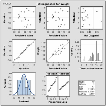
Figure 15.1: Fit Diagnostics Panel

The ODS GRAPHICS OFF statement disables ODS Graphics, and the ODS HTML CLOSE statement closes the HTML destination.

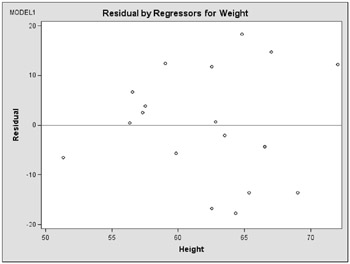
Figure 15.2: Residual Plot

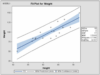
Figure 15.3: Fit Plot

Note: ODS Graphics are produced completely independently of both line printer plots and traditional high resolution graphics requested with the PLOT statement in PROC REG. Traditional high resolution graphics are saved in graphics catalogs and controlled by the GOPTIONS statement. In contrast, ODS Graphics are produced in ODS output (not graphics catalogs) and their appearance and layout are controlled by ODS styles and templates. In SAS 9.1 both line printer plots and traditional high resolution graphics requested with the PLOT statement continue to be available and are unaffected by the ODS GRAPHICS statement.

For more information about ODS Graphics available in the REG procedure, see the ODS Graphics section on page 3922 in Chapter 61, The REG Procedure.

A sample program named odsgr01.sas is available for this example in the SAS Sample Library for SAS/STAT software.

Using the ODS GRAPHICS Statement and Procedure Options

This example is taken from the Getting Started section of Chapter 36, The KDE Procedure. Here, new procedure options are used to request graphical displays in addition to the ODS GRAPHICS statement.

The following statements simulate 1,000 observations from a bivariate normal density with means (0 , 0), variances (10 , 10), and covariance 9.

  data bivnormal;   seed = 1283470;   do i = 1 to 1000;   z1 = rannor(seed);   z2 = rannor(seed);   z3 = rannor(seed);   x = 3*z1+z2;   y = 3*z1+z3;   output;   end;   drop seed;   run;  

The following statements request a bivariate kernel density estimate for the variables x and y .

  ods html;   ods graphics on;   proc kde data = bivnormal;   bivarxy/plots = contour surface;   run;   ods graphics off;   ods html close;  

A contour plot and a surface plot of the estimate are displayed in Figure 15.4 and Figure 15.5, respectively. These graphical displays are requested by specifying the ODS GRAPHICS statement prior to the procedure statements and the experimental PLOTS= option in the BIVAR statement. For more information about the graphics available in the KDE procedure, see the ODS Graphics section on page 2009 in Chapter 36, The KDE Procedure.

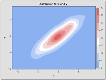
Figure 15.4: Contour Plot of Estimated Density

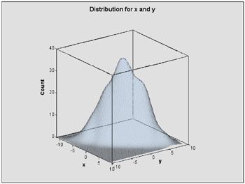
Figure 15.5: Surface Plot of Estimated Density

A sample program named odsgr02.sas is available for this example in the SAS Sample Library for SAS/STAT software.