Section 8.3. Simulation MethodologiesA Brief Review

8.3. Simulation MethodologiesA Brief Review

Prior to beginning our study of the simulation of UWB systems, we pause to review several important concepts. The three basic simulation methodologies considered here are the basic Monte Carlo technique, a modification of the Monte Carlo technique known as semi-analytic simulation, and discrete event simulation. As we use I-UWB examples throughout the discussion of these three techniques, we conclude this section with a brief discussion of the simulation of MC-UWB.

8.3.1. Monte Carlo Simulation Techniques

The most basic simulation methodology is known as Monte Carlo simulation. Monte Carlo simulation is very flexible and can be applied to any system for which the signal processing operations defined by each and every functional block in the system block diagram are known. The Monte Carlo method is a game of chance (hence the name) in which a random experiment is replicated a number of times. Monte Carlo simulation has a rich history spanning several centuries. The first application of Monte Carlo simulation of which we are aware was suggested by Laplace in 1777, who used the Monte Carlo method for estimating the value of p by using a technique known as Buffon's needle [8]. A much later application was developed in 1946 by Polish mathematician Stanislaw Ulam while pondering the probabilities of winning a game of Solitaire. Rather than mathematically computing the probability that a given 52 cards would produce a winning result, Ulam surmised that the probability could be estimated by playing the game 100 times and simply counting the number of wins [9].

All Monte Carlo simulations, including those by Laplace and Ulam, are implementations of a stochastic (random) experiment designed to estimate the probability of a particular event occurring. This is facilitated through the use of two counters in the simulation program. The first counter, known as the replication counter, measures the number of replications of the random experiment and is incremented by one each time the random experiment is repeated. The second counter, known as the event counter, is incremented by one each time the event of interest is observed. The relative frequency, or probability estimate, of the event of interest occurring is , where R and N represent the values in the event and replication counters, respectively, at the end of the simulation run.

To place this in a communications context, assume that a simulation is being performed to estimate the symbol error probability of a communications system. In this situation the underlying random experiment is the passing of a digital symbol through a communications system. This is a random experiment because channel noise, interference, or other random disturbances may, or may not, cause a transmitted symbol to be received in error. Because we are executing the simulation to estimate the symbol error probability, the event of interest is a symbol being received in error. Thus, each time a symbol is passed through the system in the simulation, the replication counter is incremented by one. Each time a transmitted symbol is received in error, the event counter is incremented by one. The simulation is assumed to process N symbols. After N symbols have been passed through the system, we calculate the relative frequency of symbol error. This relative frequency is an estimate of the symbol error probability and is given by

Equation 8.9

where N_E is the number of symbol errors observed in passing N total symbols through the simulation. The probability of symbol error is given by

Equation 8.10

Because a simulation must execute in finite time in order to be useful, the underlying random experiment can only be replicated a finite number of times. As a result, the simulation is unable to determine the probability of symbol error. The best we can do is to estimate the probability through the relative frequency. In general terms, we want the estimate to be unbiased and consistent [1]. When the estimator is unbiased and consistent, accuracy improves as the number of repetitions of the experiment increases. This also holds when simulating a system that can assume a range of parameter values, as would be the case when simulating a mobile channel. Numerous different realizations should be simulated so that a given channel realization is not treated as indicative of typical system performance.

We have seen that the disadvantage of the Monte Carlo method is that the simulation run time can be quite lengthy. This is especailly true for I-UWB systems. For example, to accurately model pulse transients, pulse distortion, and timing jitter, an I-UWB signal must often be sampled at rates much higher than the Nyquist rate. To capture ±10 ps of timing jitter, an I-UWB signal would have to be sampled at a rate sufficient to model the jitter, i.e., a minimum of one sample every 10 ps. If the inter-pulse time (time between successive pulses) is 1 µs (corresponding to a pulse repetition frequency of 1 MHz), simulating 1,000 bits means processing 100 million samples. If the UWB pulse duration is on the order of 1 ns, it is obvious that the vast majority of the simulated samples has little or no impact on the simulation results. These excess samples consume and effectively waste a significant amount of processing power and system resources. Thus, a basic trade-off exists between simulation accuracy and the time required to execute the simulation. Monte Carlo simulation is, however, ideal for simulations that involve only a small number of bits or when it is necessary to investigate the transient performance of the system.

8.3.2. Semi-Analytic Simulation Techniques

Semi-analytic simulation is a technique that mitigates the lengthy execution times frequently encountered with Monte Carlo simulation. The semi-analytic technique is applicable to any system for which the probability density function of the decision metric, such as the output of a matched filter, is known. The semi-analytic technique is most commonly applied to systems operating in a Gaussian noise environment in which the portion of the system between the point at which noise is injected and the point where the decision statistic is made is linear. The semi-analytic technique can provide results at a fraction of the time required for a Monte Carlo simulation [1].

To illustrate the semi-analytic approach, consider a UWB system operating with a Binary Pulse Amplitude Modulation waveform where we are interested in estimating the Bit Error Rate (BER). We assume that the multipath can be modeled using a tapped delay line filter, all system components are operating in a linear region, and the only noise source is thermal noise.

To set up this problem, we'll first review a few basics. Recall from digital communications theory that the BER is a function of signal space separation and noise power. Now consider the signal constellation diagram shown in Figure 8.4. In this diagram, the transmitted signal points are denoted as S₁ and S₂, the decision regions are denoted as D₁ and D₂, and f_Nx (x) is the Probability Distribution Function (PDF) of the noise in the system, modeled as a Gaussian distribution with a standard deviation of s_n. In Figure 8.4, S₁ has been transmitted, and has been received. As a result of intersymbol interference (ISI), d_x. For this receiver, a correct decision is made whenever the received signal falls in the decision region corresponding to the transmitted symbol; otherwise, an error occurs.

Figure 8.4. Diagram of a Semi-Analytic BER Estimation for BPSK.

For this system, the BER is given by

Equation 8.11

where P_E is the probability of a bit error, P_S1 and P_S2 are the probabilities that S₁ and S₂ are transmitted, and P_E|S1 and P_E|S2 are the probabilities of error given that S₁ and S₂ are transmitted, respectively. Assuming that the system noise is Gaussian gives P_E|S1 as

Equation 8.12

A similar expression defines . This can be evaluated by noting that this is the same as evaluating the Gaussian Q function at Thus, to complete the semi-analytic simulation, we must simulate to find estimates for , and s_n [1].

Furthermore, assume that the simulation sampling rate is 16 samples per symbol and the system uses transmitter filtering. The transmit filter is a fifth-order Butterworth filter and has a bandwidth equal to the symbol rate bandwidth (1/16). The simulation results for this example are shown in Figure 8.5. Notice in the left-hand pane the existence of two signal point clusters for both and due to ISI introduced in the transmitter filter (for rectangular pulse shaping a bandwidth of 2R_b (twice the bit rate) is required, whereas the filter only has a bandwidth R_b). Also notice that in this pane the two signal constellation clusters are approximately equiprobable (assuming no noise), one with a bit energy of approximately 1 and another with a bit energy of approximately (0.61)², or about 4.3 dB less than ideal. Thus, it is expected that the system would experience degradation in performance of approximately 2.15 dB, which is reflected in the right-side pane.

Figure 8.5. Binary PAM Semi-Analytic Simulation: (a) Signal Constellation Diagram, (b) Simulation Results.

8.3.3. Discrete Event Simulation Techniques

As defined in [10], a discrete event simulation is "the modeling of systems in which the [system] changes only at a discrete set of points in time." However, many simulation architectures satisfy this definition, including the Monte Carlo simulation architecture considered in Section 8.4.1. For the purposes of this discussion, we will limit discrete event simulations to those in which the system changes only at dynamically scheduled and discrete points in time. In this approach, components of our modeled system, which we will term entities, schedule future events that affect the operation of entities in the system or the operation of the simulation.

As we shall see later in this section, a discrete event simulation has several advantages over a regularly sampled simulation, including improved sampling resolution and reduced simulation runtime. Note that a discrete event simulation architecture can incorporate many different simulation techniques, including Monte Carlo and semi-analytic techniques.

Entity

An entity models a self-contained component of the system where the outputs of an entity are solely dependent on its inputs and internal parameters. An entity can model a component as complicated as a UWB receiver or as simple as an addition routine. It is convenient to think of an entity as a conceptual black box or as an object in the object oriented programming (OOP) sense. The OOP-discrete event simulation connection is especially strong, as object oriented languages like C++ and Java are frequently used for implementing discrete event simulations [10-12].

An example UWB entity represented as a UML (Unified Modeling Language) object is shown in Figure 8.6. This object implements the functionality of a UWB receiver through the use of various internal state machines, algorithms, and external interfaces. Specifically, the object maintains internal models for the antenna, amplifier, and data converter, and provides mechanisms for processing pulses and calculating BER. To use this object, the internal state machines and algorithms need not be known; only the external interfaces have to be known. As implied by this example object, the internal operations of an entity can be quite complex, depending on its model and implementation, though its interfaces can remain quite simple.

Figure 8.6. UML Diagram of a Receiver Entity.

However, developing complex entities has a number of drawbacks, including difficulties verifying the implementation and maintaining the code. To address these problems, entities can also be nested like objects. This allows entities that imply relatively complex operations, as in the receiver entity of Figure 8.6, to be constructed from a number of relatively simpler entities. These smaller entities can usually be independently developed, thus simplifying both the code verification process and later code maintenance.

For example, the Receiver entity diagrammed in Figure 8.6 could also be constructed from antenna, amplifier, data converter, and modem entities, as shown in Figure 8.7. Similarly, in a network simulation, the Receiver entity may be a nested component of a Transceiver entity, which is in turn part of a Cluster entity, which is in turn part of a Scatternet entity. Similarly, in a link simulation, Antenna, Amplifier, Data converter, and Modem entities may be comprised of a number of simpler entities.

Figure 8.7. UML Diagram of a Receiver Entity with Nested Entities.

Event

An event models an occurrence within the system at a discrete time that affects the operation of an entity or the operation of the simulation itself. The following are examples of events that alter the operation of an entity:

1. Events that spawn an entity. For instance, a simulation may treat a pulse as an entity. The pulse could be spawned by an event generated by a Transmitter entity and be later modified by Channel and Receiver entities.

2. Events that model the arrival of an input. For instance, in the preceding example, the arrival of the pulse entity at the Channel entity would be signaled by an event.

3. Events that control the operation of an entity. Continuing this example, an event could be used to change the Channel entity's SNR during a BER sweep simulation.

Events can also affect the operation of simulation itself. Typical examples of these kinds of events include the following:

1. A simulation initiation event. This event would initialize various parameters within the entities in the simulation.

2. A simulation termination event. This could be created during the simulation or scheduled before the simulation begins. The former would occur if the simulation were designed to run for a number of bit errors. The latter would occur if the simulation were designed to run a predetermined length of time.

3. An error event. Error events usually terminate simulation. Triggers for error events include missing files and incorrectly formatted inputs.

When created, an event typically includes the following information:

1. Execution time-when the event is scheduled to occur. Most events are scheduled with an additive delay to the current simulation clock time, perhaps to model processing delay or propagation delay. However, some events are scheduled at a specific time, as would be done in a simulation that runs for a predetermined length of time.

2. Target entity or entities-the entity that should handle the event. For example, in a communications link simulation, the target of a transmitted packet entity will be a single receiver entity, but in a network simulation, the target could be every Receiver entity in the network. Except in a broadcast scenario, the packet in the network simulation would be seen as interference at a number of nodes in the network that are target entities of the event though not participating in the simulated link.

3. Payload information-data being transmitted by an event. Depending on the simulation and the event, the payload could model virtually anything; a number of samples, an IP packet, or simulation control information.

4. Associated event information-information other than the payload that is associated with an event. For example, an event may include some indication of the spawning entity or error codes, should the event fail. Both would be of particular use during the debugging phase of the simulation construction.

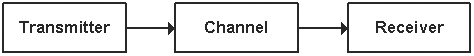
Discrete Event Simulation Operation

During normal operation, each event is triggered by an entity's response to a previous event, and the simulation continues until no events are scheduled or a simulation termination event occurs. In order to initiate the simulation, the first event must be defined. This is typically accomplished by constructing the simulation so that an initiation event occurs at the beginning of the simulation. This simulation initiation event is targeted for all extant entities in the simulation. Entities then respond to this initiation event by scheduling normal events.

During a simulation, entities are idle except when responding to events. Entities can respond to events by processing data, by adjusting parameters, and by scheduling events.

Entities may schedule events targeted for other entities, targeted for themselves, or targeted for the simulation itself. Self-scheduling is frequently done when modeling a traffic source. For example, when simulating a link employing pulse position modulation, the transmitter's traffic source can self-schedule an event corresponding to the next pulse during the processing of the current pulse.

Discrete Event Simulation Example

To illustrate the operation of a discrete event simulation, consider the canonical communications system shown in Figure 8.8 consisting of the following three components: a transmitter, a channel, and a receiver. For the purposes of this example, the system is assumed to be implementing a Binary PAM I-UWB waveform so that the transmitter generates pulses at regular intervals.

Figure 8.8. Block Diagram of a Canonical Communications System.

Assuming that the simulation is scheduled to run for 2.6 µs and pulses are generated at a nominal rate of 2 Mbps, Figure 8.9 illustrates the scheduling of events in the simulation. In this simulation, XMT is the name of the entity modeling the transmitter component, CHN names the entity modeling the channel, and RCV is the entity modeling the receiver.

Figure 8.9. Example Discrete Event Simulation Operation.

As a result of a simulation initialization event not explicitly depicted, XMT self-schedules an event at 0.0 µs to generate a pulse. In response to the 0.0 µs event, XMT schedules an event for CHN to handle the newly generated pulse and self-schedules an event at 0.5 µs to generate the next pulse. Simulation control then passes to CHN, which modifies the pulse and schedules an event for RCV at 0.6 µs. At 0.5 µs, XMT generates the second pulse, and, as before, schedules later events for CHN and for itself. Then, at 0.6 µs, RCV responds to the event corresponding to the reception of the first pulse and schedules no new events. This process continues in this manner until a simulation termination event, which is also not explicitly depicted, occurs at 2.6 µs.

This example highlights two key differences between discrete event simulations and sampled simulations:

1. In a discrete event simulation, simulation time need not progress in regularly spaced intervals. In this example, simulation time advanced at different points by 0.2 µs, 0.3 µs, and 0.1 µs.

2. In a discrete event simulation, processing control is not linear. To handle these dynamic situations, a more complex structure is required to support the construction of discrete event simulations.

Discrete Event Simulation Development

In addition to events and entities, most discrete event simulations contain at least two additional components-an event manager and an event list.

An event manager is minimally responsible for the following simulation tasks:

1. Generating the initial simulation event.

2. Passing control to the proper entity at the scheduled event time.

3. Handling error events.

4. Resolving event-scheduling conflicts.

Scheduling conflicts can occur when two entities schedule events for the same time. This can be resolved in a number of different ways, but the most common technique is a first-come-first-serve approach, i.e., the event that was scheduled first is handled first.

Additionally, the event manager may provide additional services, such as supplying current simulation time and collecting statistics, provided that the current simulation time is particularly convenient for entities scheduling events, but this is not a necessity. Statistics could alternately be collected by each modeling entity or collected by special statistics entities.

To aid the event manager in these tasks, an event list is typically implemented. The event list is ordered by scheduled execution time, with the event scheduled for current execution placed at the head of the list, and the event scheduled farthest in the future placed at the tail of the list. Newly created events are inserted by timestamp into the list; completed events are deleted from the list. Although it represents poor programming practice, newly created events with timestamps before the list head are generally discarded. As a side benefit of an event list, the implementation of a simulation clock is relatively straightforward, as the current simulation time can be taken from the timestamp of the event at the head of the list.

Simulation operation with an event manager then proceeds by the repetition of the following steps until a termination event occurs or the list is empty:

1. Execute the event at the top of the event list. We call this event A.

2. Insert any new events spawned by A into the event list.

3. Set the list head pointer to the event immediately after A.

Revisiting our example from Figure 8.9, Figure 8.10 depicts how an event list for the simulation would appear at three different instances of time. At 0.0 µs the simulation initiation event and the simulation termination events are scheduled. At 0.2 µs, an event at the XMT entity, which also generated the first pulse, has scheduled events for the CHN and XMT entities at 0.2 µs and 0.5 µs respectively. (Note that these two events have been inserted into the list ahead of the previously scheduled termination event.) Then at 1.6 µs, four events have been scheduled: one for the RCV to receive the third pulse, one for the CHN entity to process the fourth pulse, one for the XMT entity to generate the fifth pulse, and the simulation termination event.

Figure 8.10. Event Lists at Selected Simulation Times for a Discrete Event Simulation.

Discrete Event Simulation Performance Considerations

A discrete event simulation architecture offers several performance advantages over a traditional sampled continuous time simulation due to the possibility of a higher sampling resolution and shorter simulation run time. To illustrate why this is so, consider the pair of pulses that might be generated from a Saleh-Valenzuela channel model as applied to a BPSK I-UWB waveform, as depicted in Figure 8.11.

Figure 8.11. UWB Signal Generated Using Saleh-Valenzuela Channel Model.

In this waveform, a pulse arrives at the receiver with significant energy over the period T_p that is significantly less than the frame period, T_f, allotted for the pulse and thus has a simulation duty cycle of r =T_p/T_f. For this particular channel realization, there are ten significant multipath components. If the multipath components arrived at regular intervals, a uniform sampling rate simulation would require a sampling rate of T_p/10 and have a total of 10/r samples per frame. However, a discrete event simulation^[1] would require just ten samples for the entire frame. This represents, at least potentially, an enormous savings for low duty-cycle waveforms.

^[1] The discrete event simulation could be constructed so that the channel generates 10 events for the receiver, or the channel could generate a single 10 sample event for the receiver. Ignoring simulation overhead, the nominal number of processing cycles would be the same.

Now consider the more likely scenario wherein the multipath components are irregularly spaced with minimum spacing of Dt. A uniform sampling architecture requires 1/rDt samples to provide sufficient resolution. For a little perspective, this value will necessarily be greater than or equal to the previous total of 10/r samples per frame, and in many cases significantly greater. However, the discrete event simulation still only requires 10 samples per frame. As this example demonstrates, constructing a UWB simulation using a discrete event simulation architecture can provide significant improvements in both time resolution and simulation run-time.

However, it should be noted that this analysis overlooked some penalties that must be incurred by a discrete event simulation. In particular, processor cycles are lost handling events. In a discrete event simulation, processor cycles are lost in the following places:

1. The exchange of simulation control between the event manager and entity.

2. The handling of events within an entity.

3. The management of the event list.

Thus, the processing gain seen by implementing a discrete event simulation is lower in an actual implementation than predicted by a theoretical implementation. However, for low duty-cycle simulations, discrete event simulations retain the potential to significantly outperform a uniform sampling scheme.

Another drawback to a discrete event simulation architecture is increased development time. Many familiar communications simulation languages, such as Matlab, do not offer built-in discrete event simulation support. To use these languages, some additional work has to be performed to implement the event manager and event list. Additionally, the construction of an entity interface is slightly more complicated, as additional processing must occur to handle incoming events and to schedule outgoing events.

8.3.4. Multicarrier UWB (MC-UWB) Simulation

Previously, we saw that the following difficulties are encountered when simulating I-UWB systems:

1. Many traditional modeling parameters, such as phase, have an unclear meaning in a wide bandwidth signal.

2. Many traditional modeling approaches, such as complex baseband and I-Q representation, are not applicable to I-UWB.

3. Traditional channel noise modeling assumptions break down due to multipath resolvability.

4. Channel parameters, such as gain and group delay, are frequency variant.

5. The UWB necessitates an ultra-high sampling rate.

However, as an MC-UWB signal consists of numerous narrowband signals, the majority of these issues are not problems for MC-UWB simulation. Phase can be readily defined for each carrier in an MC-UWB signal. Each carrier signal in an MC-UWB can be readily broken into I-Q components and modeled using a complex baseband representation. Because of the narrow bandwidth of each carrier signal, fewer multipaths are resolvable, so traditional Gaussian, Rayleigh, and Rician noise models can often be assumed. Within each band, gain and group delay should be relatively frequency invariant. Further, as an MC-UWB signal is continuously transmitted, the familiar sampled continuous time Monte Carlo architecture can be implemented for MC-UWB simulations. Thus, a MC-UWB simulation is not significantly troubled by four of the major difficulties encountered in an I-UWB simulation.

However, as Nyquist requires, there is no avoiding the use of an ultra-high sampling rate for simulating UWB's ultra-high bandwidth. Also, because an MC-UWB signal is a continuous signal, a discrete event architecture is not appropriate and cannot be expected to produce a significant savings in processing resources.

There are also some issues that are more critical to the operation of a MC-UWB system than to an I-UWB system and serve as sources of difficulty for MC-UWB simulation. Most notable of the issues is MC-UWB's high peak-to-average power ratio (PAPR). Because of high PAPR, MC-UWB devices are repeatedly driven into nonlinear regions. This creates the following two issues for MC-UWB simulation:

1. As semi-analytic simulation techniques typically assume a linear system after the point of noise injection, there can be significant difficulty in implementing a semi-analytic simulation. Thus Monte Carlo techniques are generally preferable for MC-UWB simulations.

2. More complex component models must be used to ensure that these nonlinear effects are properly captured by the simulation. Accordingly, Section 8.4 presents an extended discussion of component models for UWB communication systems with a particular focus on modeling nonlinear effects.