Denormalizing the Database

After a database has been normalized to the third form, database designers intentionally backtrack from normalization to improve the performance of the system. This technique of rolling back from normalization is called denormalization. Denormalization allows you to keep redundant data in the system, reducing the number of tables in your schema and reducing the number of joins to retrieve data.

TIP

Duplicate data is more helpful when the data does not change very much, such as in data warehouses. If the data changes often, keeping all "copies" of the data in sync can create significant performance overhead, including long transactions and excessive write operations.

Denormalization Guidelines

When should you denormalize a database? Consider the following points first:

• Be sure you have a good overall understanding of the logical design of the system. This knowledge helps in determining how other parts of the application are going to be affected when you change one part of the system.

• Don't make an attempt to denormalize the entire database at once. Instead, focus on the specific areas and queries that are accessed most frequently and are suffering from performance problems.

• Understand the types of transactions and the volume of data associated with specific areas of the application that is having performance problems. You can resolve many such issues by tuning the queries without denormalizing the tables.

• Determine whether you need virtual (computed) columns. Virtual columns can be computed from other columns of the table. Although this violates third normal form, computed columns can provide a decent compromise because they do not actually store another exact copy of the data in the same table.

• Understand data integrity issues. With more redundant data in the system, maintaining data integrity is more difficult and data modifications are slower.

• Understand storage techniques for the data. Using RAID and SQL Server filegroups may improve performance without denormalization.

• Determine the frequency at which data changes. If the data is changing too often, the cost of maintaining data and referential integrity might outweigh the benefits provided by redundant data.

TIP

If you are experiencing severe performance problems, denormalization should not be the first step you take to rectify the problem. Identify specific issues that are causing performance problems. Usually, you will discover factors such as poorly written queries, poor index design, inefficient application code, or poorly configured hardware. You should try to fix such issues before taking steps to denormalize database tables.

Essential Denormalization Techniques

You can employ various methods to denormalize a database table and achieve desired performance goals. Some of the useful techniques used for denormalization include the following:

• Keeping redundant data and summary data

• Using virtual columns

• Performing horizontal data partitioning

• Performing vertical data partitioning

Redundant Data

Joins are inherently expensive in a relational database from an I/O standpoint. To avoid common joins, add redundancy to the table by keeping exact copies of the data in multiple tables. The following example demonstrates this point. The example shows a three-table join to get the title of a book and the primary authors' name :

 select c.title,         a.au_lname,        a.au_fname    from   authors a join titleauthor b on a.au_id = b.au_id    join titles c on b.title_id = c.title_id    where  b.au_ord = 1    order by c.title 

You could improve the query performance for this example by adding the columns for the first and last name of the primary author to the titles table itself and storing the information in the titles table directly. This will eliminate the joins altogether. Here is what the revised query would look like if this denormalization technique were implemented:

 select title,         au_lname,        au_fname    from  titles    order by title 

As you can see, the au_lname and au_fname columns are now redundantly stored in two places: the titles table and the authors table. It is obvious that with more redundant data in the system, maintaining referential integrity and data integrity is more difficult. For example, if the author's last name changed in the authors table, to preserve data integrity, you must also change the corresponding au_lname column value in titles table to reflect the correct value. You could use SQL Server triggers to maintain data integrity, but recognize that update performance could suffer dramatically. For this reason, it is best if redundant data is limited to data columns whose values are relatively static and are not modified often. In the example presented, it is highly unlikely that an author's last name for a published book would change.

Computed Columns

A number of queries calculate aggregate values derived from one or more columns of a table. Such computations can sometimes be CPU intensive and can have an adverse impact on performance if they are performed frequently. One of the techniques to handle such situations is to create an additional column that stores the computed value. Such columns are called virtual columns or contrived columns. Starting with SQL Server 7.0, computed columns are natively supported. You can specify such columns during create table or alter table commands. The following example demonstrates the use of computed columns:

 create table emp (          empid int not null primary key,         salary money not null,         bonus money not null default 0,         total_salary as ( salary+bonus )         ) go insert emp (empid, salary, bonus) values (100, 0000.00, 000) go select * from emp go empid       salary         bonus                total_salary ----------- -------------  -------------------- ---------------- 100         150000.0000    15000.0000           165000.0000 

Virtual columns are not physically stored in SQL Server tables. SQL Server internally maintains a column property iscomputed in the system table syscolumns to determine whether a column is computed. The value of the virtual column is calculated at the time the query is run. Computed columns cannot pull data from more than one table, however, so if this is required, you must create a physical column and use stored procedures or triggers to generate and maintain its value.

In SQL 2000, computed columns can participate in joins to other tables, and they can be indexed. Creating an index that contains a computed column creates a physical copy of the computed column in the index tree. Whenever a base column participating in the computed column changes, the index must also be updated, which adds overhead and possibly slows down update performance.

Summary Data

Summary data is most helpful in a decision support environment. To satisfy reporting requirements, calculate sums, row counts, or other summary information and store it in a separate table. You can create summary data in a number of ways:

• Real time ”Every time your base data is modified, recalculate the summary data using the base data as a source. This is typically done using stored procedures or triggers.

• Real time incremental ”Every time your base data is modified, recalculate the summary data using the old summary value and the new data. This is more complex, but it could save time if the increments are relatively small compared to the entire data set. This too is typically done using stored procedures or triggers.

• Delayed ”Use a scheduled job to recalculate summary data on a regular basis. This is the recommended method to use in an OLTP system to keep update performance optimal.

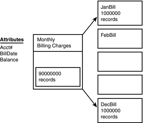
Horizontal Data Partitioning

As tables grow larger, data access time also tends to increase. For queries that need to perform table scans , the query time is proportional to the number of rows in the table. Even when you have proper indexes on such tables, access time slows as the depth of the index trees increase.

The solution is splitting the table into multiple tables such that each table has the same table structure as the original one but stores a different set of data. Figure 39.1 shows a billing table with 90 million records. You can split this table into 12 monthly tables (each with an identical table structure) to store billing records for each month.

Figure 39.1. Horizontal partitioning of data.

You should carefully weigh the options when performing horizontal splitting. Although a query that only needs data from a single month gets much faster, other queries that need a full year's worth of data become more complex. Also, queries that are self-referencing do not benefit much from horizontal partitioning. For example, the business logic might dictate that each time you add a new billing record to the billing table, you need to check any outstanding account balance for previous billing dates. In such cases, before you do an insert in the current monthly billing table, you must check the data for all the other months to find any outstanding balance.

TIP

Horizontal splitting of data is useful where a subset of data might see more activity than the rest of the data. For example, in a healthcare provider setting, 98 percent of the patients are inpatients and only 2 percent are outpatients. In spite of the small percentage involved, the system for outpatient records sees a lot of activity. In this scenario, it makes sense to split the patient table into two tables, one for the inpatients and one for the outpatients.

When splitting tables horizontally, you must perform some analysis to determine the optimal way to split the table. Try to find a logical dimension along which to split the data. The best choice will take into account the way your users use your data. In the previous example, date was mentioned as the optimal split candidate. However, if your users often did ad hoc queries against the billing table for a full year's worth of data, they would be unhappy with your choice to split that data among 12 different tables. Perhaps a customer type or other attribute would be more useful.

NOTE

With support for partitioned views in SQL Server 2000, you can hide the horizontal splitting of the tables by defining a partitioned view on the tables. The benefit of partitioned views is that multiple horizontally split tables will appear to the end users and applications as a single large table. When properly defined, the optimizer will automatically determine which tables in the partitioned view need to be accessed and will avoid searching all tables in the view. The query will run as quickly as if it were run only against the necessary tables directly. For more information on defining and using partitioned views, see Chapter 27, "Creating and Managing Views in SQL Server."

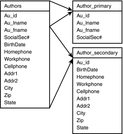
Vertical Data Partitioning

As you know, a database in SQL Server consists of 8KB pages, and a row cannot span across multiple pages. Therefore, the total number of rows on a page depends on the width of a table. This means the wider the table, the fewer the number of rows per page. You can achieve significant performance gains increasing the number of rows per page, which in turn reduces the number of I/Os on the table. Vertical splitting is a method of reducing the width of a table by splitting the columns of a table into multiple tables. Usually, all frequently used columns are kept in one table and others are kept in the other table. This way, more records can be accommodated per page, fewer I/Os are generated, and more data can be cached into SQL Server memory. Figure 39.2 illustrates a vertically partitioned table. The frequently accessed columns of the authors table are stored in the author_primary table, whereas less frequently used columns are stored in the author_secondary table.

Figure 39.2. Vertical partitioning of data.

TIP

Make the decision to split data very carefully, especially when the system is already in production. Changing the data structure might have a system-wide impact on a large number of queries that reference the old definition of the object. In such cases, to minimize risks, SQL Server views can be effective in hiding the vertical partitioning of data. Also, if you find that users and developers are frequently joining between the vertically split tables because they need to pull data together from both tables, you might want to reconsider the split point or the splitting of the table itself. Frequent joins between split tables with smaller rows will require more I/Os to retrieve the same data than if the data resided in a single table with wider rows.

Performance Implications of Zero to One Relationships

Suppose that one of the development managers in your company, Bob, approaches you to discuss some database schema changes. He is one of several managers whose groups all use the central User table in your database. Bob's application makes use of about 5 percent of the users in the User table. Bob has a requirement to track five yes/no/undecided flags associated with those users. He would like you to add five, one-character columns to the user table to track this information. What do you tell Bob?

Bob has a classic zero-to-one problem. He has some data he needs to track, but it applies to only a small subset of the data in the table. You can approach this problem in one of three ways:

• Option one: Add the columns to the User table ”95 percent of your users will have NULL values in those columns, and the table will become wider for everybody.

• Option two: Create a new table with a vertical partition of the User table ”The new table will contain the User primary key and Bob's five flags. 95 percent of your users still have NULL data in the new table, but the User table is safe from the effects of this. Because other groups don't need to use the new partition table, this is a nice compromise.

• Option three: Create a new vertically partitioned table as in option two, but populate it only with rows that have at least one non-NULL value for the columns in the new partition ”This is great for database performance, and searches in the new table will be wonderfully fast. The only drawback to this is that Bob's developers will have to add additional logic to their applications to determine if a row exists during updates. Bob's folks will need to use an outer join to the table to cover the possibility that a row doesn't exist.

Depending on the goals of your project, any one of these options is appropriate. The first option is simple and is the easiest to code for and understand. The second option is a good compromise between performance and simplicity. The third option gives the best performance in certain circumstances, but impacts performance in certain other situations and definitely causes more coding work to be done.