Chapter IV: Hierarchies

Elaheh Pourabbas, Istituto di Analisi dei Sistemi ed Informatica – C. N. R.

Italy

Maurizio Rafanelli, Istituto di Analisi dei Sistemi ed Informatica – C. N. R.

Italy

In this chapter we will focus on the rules of aggregation hierarchies in analysis dimensions of a cube. We give an overview of the related works on the basic concepts of the different types of aggregation hierarchies. We then discuss the hierarchies from two different points of view: mapping between domain values and hierarchical structures. In relation to them, we introduce the characterization of some OLAP operators on hierarchies and give a set of operators that concern the change in the hierarchy structure. Finally, we propose an enlargement of the operator set concerning hierarchies.

INTRODUCTION

Hierarchies play a fundamental role in knowledge representation and reasoning. They have been considered as the structures created by abstraction processes. According to Smith & Smith (1977), an abstraction process is an instinctively known human activity, and abstraction processes and their properties are generally used for multi-level object representation in information systems. An abstraction of a system is a model of that system in which certain details are deliberately omitted with the objective of allowing users to notice details of the system which are relevant to the application, but ignore other details and consequently simplify the model.

Sometimes, a system may have too many relevant details for a single abstraction to be intellectually manageable. However, manageability can be provided by decomposing the model into a hierarchy of abstraction. One advantage of this hierarchy of abstraction is the capability of accessing the model at different levels of abstraction.

An abstraction of an object denotes its essential characteristics which distinguish it from all other objects. It can be defined as a mental ordering imposed on the environmental model depending on the goal or task of the user. An abstraction can be understood as a selection of a set of attributes, objects, or actions from a much larger set of attributes, objects, or actions according to certain criteria determined by the above-mentioned goal or task. Repeating this selection several times, that is, continuing to choose, from each subset of objects, another subset of objects with even more abstract properties, we create other levels of (semantic) details of objects. In Smith & Smith (1977), two kinds of abstraction are defined. The former, called aggregation, refers to an abstraction in which a relationship between objects is regarded as a higher level object. The latter, called generalization, refers to an abstraction in which a set of similar objects (i.e., a class of objects) is regarded as a generic object.

The complete structure created by the abstraction process is a hierarchy, and the type of hierarchy depends on the operation used for the abstraction process and the relations. As for the relations the best known in the literature are classification, generalization, association (or grouping), and aggregation. Their main characteristics are briefly listed in the following.

Classification is a simple form of data abstraction in which an object type is defined as a set of instances. It introduces an instance-of relationships between an object type in a schema and its instances in the database.

Generalization is a form of abstraction in which similar objects are related to a higher level generic object. It forms a new concept by leaving out the properties of an existing concept. With such an abstraction the similar constituent objects are specializations of the generic objects. At the level of the generic object, the similarities of the specializations are emphasized, while the differences are suppressed. This introduces an is-a relationship between objects. The is-a relation between types is a partial order and organizes types into an is-a hierarchy. This relation covers a wide range of categories which are used in other frameworks, such as inheritance, implication, and inclusion. It is the most frequent relation resulting from subdividing concepts, called taxonomies in lexical semantics. The inverse of the generalization relation, called specialization, forms a new concept by adding properties to an existing concept.

A particular type of generalization hierarchy, named filter hierarchy, is defined by the so-called filtering operation. This operation applies a filter function to a set of objects on one level and generates a subset of these objects on a higher level. The main difference from the generalization hierarchy is that the objects that do not pass the filter will be suppressed at the higher level.

Association or grouping is a form of abstraction in which a relationship between member objects is considered as a higher level set of objects. With this relationship the details of member objects are suppressed and properties of the set object are emphasized. This introduces the member-of relationship between a member object and a set of objects.

Aggregation is a form of abstraction in which a relationship between objects is considered as a higher level aggregate object. Each instance of an aggregate object can be decomposed into instances of the component objects. This introduces a part-of relationship between objects. The type of hierarchy constructed by this abstraction is called an aggregation hierarchy.

Like data warehousing and OLAP, the above-mentioned aggregation hierarchies are widely used to support data aggregation. Thus, an aggregation hierarchy is an effective form of knowledge representation for encoding prior domain knowledge relevant to a data cube. In a simple form, such a hierarchy shows the relationships between domains of values. Each operation on a hierarchy can be viewed as a mapping from one domain to a smaller domain. In the OLAP environment, hierarchies are used to conceptualize the process of generalizing data as a transformation of values from one domain to values of another smaller/bigger domain by means of drill-down/roll-up operators.

In this chapter, attention will be focused on the rules of aggregation hierarchies in analysis dimensions of a data cube. In this context, some different types of hierarchies, as well as their characterization, will be discussed. These hierarchies divide a single dimension into different levels of aggregation. In relation to them, we discuss the characterization of some OLAP operators which refer to hierarchies in order to maintain data cube consistency. Moreover, we propose a set of operators for changing the hierarchy structure. The issues discussed provide modeling flexibility during the schema design phase and correct data analysis.

The chapter is structured as follows: the next section gives an overview of the related works on the basic concepts of the different types of aggregation hierarchies. We then discuss the hierarchies from two different points of view: mapping between domain values and hierarchical structures. The next section introduces the characterization of some OLAP operators on hierarchies and gives a set of operators that concern the change in the hierarchy structure. We then proposes an enlargement of the operator set concerning hierarchies, and conclude the chapter.

Related Works

The core of the aggregation hierarchy revolves around the partial order, a simple and powerful mathematical concept to which a lot of attention has been devoted (see Birkhoff, 1979; Davey & Priestley, 1993). The partial ordering can be represented as a tree, with the vertices denoting the elements of the domains and the edges representing the ordering function between elements. The notion of levels has been introduced through the idea that vertices at the same depth in the tree belong to the same level of the hierarchy. Thus, the member of levels in the hierarchy corresponds to the depth of the tree. The highest level is the most abstract of the hierarchy and the lowest level is the most detailed.

A partially ordered set is a pair (V, ≤) where V is a set and ≤ is a reflexive, anti-symmetric, and transitive binary relation defined on. Accordingly, the concept of hierarchy can be sketched by the following definition V:

Definition: A hierarchy is an ordered structure, where the order is established between individuals or between classes of individuals; the ordering function may be any function defining a partial order:

A vertex v₁ in a graph is on a lower level than v₂ if and only if there exists a function f, such that v₂ can be calculated by applying f to a set of v_i of which v₁ is a member. The function f must be reflexive, anti-symmetric, and transitive.

Now, suppose that T is a subset of V. Then, t∊ T is a maximal element of T if t ≤ x ∊ T implies that t = x, and t is the greatest element of T if t ≥ x for each x ∊ T. Minimal and least elements can be defined dually. If V has one minimal (maximal) element, then it will be called the bottom (top) and it is usually indicated by ⊥(T).

As in data warehousing and OLAP, the notion of partial ordering is widely used to organize the hierarchy of different levels of data aggregation along a dimension. Sometimes, hierarchies have been perceived structurally as trees, i.e., no generic object is the immediate descendant of two or more generic objects, and where the immediate descendants of any node (supposing any hierarchy is represented by a graph) have classes which are mutually exclusive. A class with a mutually exclusive group of generic objects sharing a common parent is called a cluster. Generally speaking, many real cases cannot be modeled by the hierarchies having the previous characteristics. For instance, in Figure 1 two illustrative examples of this situation are shown.

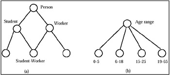
Figure 1: Examples of non-hierarchical structures

For this reason, usually, a dimension hierarchy is represented as a direct acyclic graph. Sometimes, it can be defined with a unique bottom level and a unique top level, denoted by ALL (see Gray et al., 1997).

One of the most important issues related to the aggregation hierarchy is the correct aggregation of data, and this has been considered since 1980 (see Chen & Shoshani, 1981; Rafanelli & Shoshani, 1990; Lenz & Shoshani, 1997). It is known as summarizability, which intuitively means that individual aggregate results can be combined directly to produce new aggregate results.

Rafanelli & Shoshani (1990), speaking on the Statistical Object Representation Model (STORM), give some concepts and definitions regarding the summarizability of a category attribute (for a given statistical object, the term by which they denote a multidimensional aggregate data, MAD), the fullness and completeness of a mapping between category attributes which belong to the same hierarchy (represented in the graphical model by nodes labeled C, so that this mapping is called C-mapping), and finally, the well-formedness of a MAD.

Some observations on null values are made and the "unknown" and "non-existing" values are studied. In particular, in the former (unknown) case, the total with respect to the category attribute, for which there are unknown values, is not the total of the attribute itself. In the latter (non-existing) case, although it is true that, for example, the total number of cancer of the prostate cases is the total reported in the marginal (summarizing with regard to "sex"), the information on these cases are the total number of males alone and not the entire population is lost. For this reason, for the summary data of the tables in output, the authors distinguish two null values: non-available value (symbol "NA") and structural zero (symbol "-").

Structural zeros are also important in the case in which the cross-product among the different category attributes which describe the summary data is incomplete (for example, in the case of a relation). Suppose we have the MAD Occupation in the Computer Science Department in 1990 at UCLA, and suppose that the structure of this department is the following: <Research, Technical, Administrative>. Moreover, suppose that the Professional/ Academic titles admitted for each area are respectively <PhD, Degree>, <PhD, Degree, Diploma (General Certificate of Education)>, and <Degree, Diploma (General Certificate of Education)>. This situation is shown in Figure 2 by a bipartite graph and by a G-relation (discussed in Chapter 2 and proposed in Su, 1983), where the last column is the summary data. Therefore, the authors, after having defined the classification instance as a C-mapping between one category attribute instance of the higher level and one or more category attribute instances at the lower level, give the following definitions:

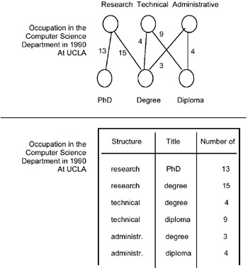
Figure 2: Example of the MAD occupation

Definition: A classification instance is full if all the category attribute instances of the lower level exist (according to the semantics of the classification as determined by the database administrator).

Note that fullness is a semantic concept.

Corollary: A C-mapping is full if each classification instance is full.

As an example, the authors consider the mapping between the two category attributes "city" and "state" of the hierarchy "Political classification." In order to summarize correctly over cities, they observe that it is necessary to know that there are no missing values in its definition domain. However, it is also reasonable to assume that some small towns or other villages were not included in the list of cities. In this case the summarization from city to state level will have incorrect results. To compensate for such situations, often the instance "other" is included in the definition domain.

The graphical conceptual STORM model uses nodes to represent a MAD structure. In particular, it uses one S node to represent the summary values of the MAD (its measure), one A node to represent the cross-product among the different category attributes (i.e., the descriptive space of the MAD) which describe the measure, and C nodes to represent the category attributes mentioned above. Non-oriented edges link two nodes (in the case of a hierarchy, the edges consist of double lines).

The authors define the S-mapping as the mapping between an A node and the relative S node (i.e., between a tuple of the descriptive space of the MAD and the corresponding measure instance); then, they give the definitions of completeness, quasi-completeness, and incompleteness of an S mapping as follows:

Definition: An S-mapping is complete if for every tuple of values in A a unique, defined (i.e., not "non-available" or "structural zero") value in S exists.

Definition: An S-mapping is quasi-complete if for some tuple in A a "structural zero" exists, that is a non-existent value (represented by "-" in the summary attribute) in S.

For example, in a database on cancer rates, a value for prostate cancer for females (regardless of any other category attributes) does not exist.

Definition: An S-mapping is incomplete if for every tuple of values in A a unique, defined, or non-available (represented by "NA" in the summary attribute) value in S exists.

Note that an incomplete S-mapping can become complete (for example, it may be that not all the data referring to a given fact is available at present, but within a given time they will all be available).

They give the definition of a summarizable category attribute in the following way:

Definition: A category attribute of a given MAD is summarizable if:

1. there is no overlapping among the values of its definition domain;

2. there is no overlapping among the numeric values of the summary attribute;

3. there is no overlapping along the time dimension among the population (people, cars, etc.) considered in the phenomenon studied by this statistical object;

4. the edge starting from it, if it takes part of a classification hierarchy, defines a complete C-mapping toward the upper level C node;

5. the unit of measure is the same for each instance of the definition domain and for each category attribute of a possible partition of which it takes part;

6. no unknown (NA, not available) value appears in the summary attribute.

For a clear description of the above-mentioned cases, we give an example for each of them:

Case A: Suppose we have a statistical object in which the examined phenomenon is "people with a given disease," and that this phenomenon is classified by "state," "sex," and "disease." For a given state and a given sex, the total number of people that had at least one disease can be lower than the total obtained from the sum of the number of people that had a given disease (it is sufficient to think of a person that had two or more diseases).

Case B: Suppose we have a statistical object in which a category attribute is, for example, "age range." If the domain instances are, for example, < 0–10, 6–18, 19–29, 30–60, over 60 >, an overlapping among these values exists. This fact does not necessarily determine an overlapping among the numeric values of the summary attribute (we do not know if, with regard to this statistical object, somebody exists in the range "6–10"), but not knowing it determines the non-summarizability of the category attribute.

Case C: It is sufficient to consider, for this case, two different time series which describe, over the years, the different phenomena "Production of cars" and "Moving cars," by model. In the former there is no overlapping, but in the latter a large number of cars which moved in a given year, move also during the following year, and so on.

Case D: This is the case in which a sub-area of a category attribute is completely lacking (for example, all the states of "west" in the statistical object "Car production" by "year" and "state"); obviously the summarization of the category attribute "state" will not be possible with regard to the upper C node "country," even if, in general, it will be possible, by an estimation based on more or less complex criteria, to evaluate the lacking values. Another situation is the classification hierarchy "state"-"city," in the statistical object "Population of the USA" by state and year. If only the population of San Francisco and Los Angeles appears in the statistical object, we cannot summarize "city" because the population of California obtained in such a way would be an erroneous value.

Case E: This is the case of the category attribute "dairy" in which you can have two definition domains, each of them with different units of measure.

Case F: In this case, non-available (NA) values appear in the summary attribute of a statistical object as "holes" (for example, we can have car production in California for the years 1985, 1986, 1987, and 1990, but do not have it for the years 1988 and 1989. Therefore, the value of the production of cars in California for the years 1985–1990 is "NA"). This situation is like the previous Case D, and it is also generally solved by estimated values (for example, by an interpolation).

The authors give the definition of well-formedness MAD, based on the previous concept of summarizability:

Definition: A MAD is well formed if each of its category attributes is summarizable.

As subsequently discussed in Lenz & Shoshani (1997), summarizability of OLAP and multidimensional aggregate databases is an extremely important property because violating this condition can lead to erroneous conclusions and decisions. The summarization operation inherits the concept proposed in Rafanelli & Shoshani (1990) and discussed above. It can reduce the dimensions of the multidimensional space of a MAD when the dimension consists of a simple category attribute (without a hierarchy, for example, race or sex), or cannot reduce it when the summarization is carried out along the same dimension (i.e., when a hierarchy exists), thus decreasing the granularity of this dimension.

Summarizability conditions are the conditions under which the summarization operation produces the correct result. Suppose we have applied the aggregation process described in Chapter 2 to a relational (micro) database. In this way the characteristics of all the multidimensional aggregate data (MAD) of the multidimensional aggregate database are defined (i.e., name of each fact described by each MAD and belonging phenomenon, their summary type, their base relation (i.e., their descriptive space), their subject, etc.). The authors affirm that three necessary conditions of summarizability have to be satisfied:

1. Disjointness of the category attributes: The disjointness condition means that the category attributes must form disjoint subsets over the individuals/objects. Note that the testing of this disjointness condition is carried out at the instance level of the microdata. This condition is shown schematically in Figure 3(a), where the broken line violates the disjointness condition. It is necessary to examine this condition for two different cases: a category attribute that is part of the multidimensional space (the category attribute is a leaf node), and a category attribute that belongs to a classification hierarchy only (the category attribute is a non-leaf node). In the former, the disjointness test is relative to the individuals of the "microdata framework." In the latter, the non-leaf nodes form a category hierarchy, so that the disjointness test is made relative to the node below it. For example, in the hypothetical hierarchy "state-city," "state" is a non-leaf node, so that we have to test whether states form disjoint sets over cities. If it turns out that cities have globally unique names, this condition holds, but if cities do not have unique names (i.e., the same city name is sometimes used in two or more states), this summarizability condition is violated.

   
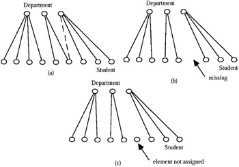
   Figure 3: Example of non-completeness

2. Completeness: Another summarizability condition to verify is whether the grouping of individuals/objects into clusters is "complete." The test for completeness in this context has two parts. The first is to verify that all the elements of the clusters exist (i.e., the union of all clusters constitutes the entire set of the individuals/objects). The second is to verify that each individual/object is assigned to a category. These two parts of the test are shown schematically in Figures 3(b) and (c). An important aspect of this condition is that it depends on the summary attribute. As was the case for Condition 1, the tests for the two types of category attributes (i.e., leaf and non-leaf nodes) are different.

3. Summary type of the individual/object measure: Summarization is performed quite differently with temporal categories as opposed to non-temporal ones. Summary attributes can be classified either as a flow (or rate), a stock (or level), or a value-per-unit. Flows refer to periods and are recorded at the end of these periods (they record the cumulative effect over a period), while stocks are measured and recorded at particular points in time. Value-per-units are determined by a fixed time, too, but are not similar to stocks in so far as their unit is different. While temporal summarizability of flows is semantically meaningful, temporal summarizability for stocks and value-per-unit depends on the aggregation function being applied.

The effects of the type of function and the type of attribute on temporal summarizability is shown in Figures 4 (by the type of function and summary attribute) and 5 (non-temporal summarizability dependent upon type of function and attribute).

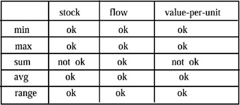
Figure 4: Temporal Summarization by Function and Summary Attribute Type

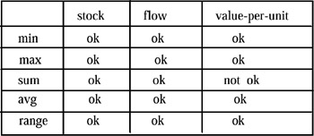
Figure 5: Non Temporal Summarization by Function and Summary Attribute Type

In conclusion, the third condition of summarizability checks for the compatibility of the three parts of a summarization function: the category attribute, the summary attribute, and the aggregation function. It is necessary to determine the category attribute type (temporal, non-temporal), the summary attribute type (stock, flow, value-per-unit), and determine whether summarizability holds for the aggregation function associated with the MAD.

More recently, the problem of heterogeneity in aggregation hierarchy structures and its effect on data aggregation has attracted the attention of the OLAP database community. The term heterogeneity, as introduced by Kimball (1996), refers to the situation where several dimensions representing the same conceptual entity, but with different categories and attributes, are modeled as a single dimension. According to this description, which has also been called multiple hierarchy (see Agrawal, Gupta, & Sarawagi, 1997; Pourabbas & Rafanelli, 2000), dimension modeling may require every pair of elements of a given category to have parents in the same set of categories. In other words, the roll-up function between adjacent levels is a total function. The hierarchies with this property are known to be regular or homogeneous. For instance, in a homogeneous hierarchy, we cannot have some cities that roll-up to provinces and some to states, i.e., the roll-up function between City and State is a partial function.

In order to model these irregular cases, some authors introduced heterogeneous dimensions. For instance, the city Washington, DC, cannot roll-up to State because it rolls-up to Country without passing through State. In the context of irregular or heterogeneous hierarchies, there are several solutions which deal with summarizability.

Lehner, Albrecht, & Wedekind (1998) tackled heterogeneity by proposing different solutions. Their proposal consists of transforming heterogeneous dimensions into homogeneous dimensions in order to be in Dimensional Normal Form (DNF). This transformation is actually performed by considering categories, which cause the heterogeneity, as attributes for tables outside the hierarchy. On the flattened child/parent relation, summarizability is achieved for dimension instances.

Pederson & Jensen (1999) considered a particular class of heterogeneous hierarchies, for which they proposed their transformation into homogeneous hierarchies by adding null members to represent missing parents. In their opinion, summarizability occurs when the mappings in the dimension hierarchies are onto (all paths from the root to a leaf in the hierarchy have equal lengths), covering (only immediate parent and child values can be related), and strict (each child in a hierarchy has only one parent). Other conditions required for summarizability are that the relationships between facts and dimensions are many-to-one and that facts are always mapped to the lowest level in the dimensions. The proposed solutions consider a restricted class of heterogeneous dimensions, and null members may cause a waste of memory and increase the computational effort due to the sparsity of the cube views.

Hurtado & Mendelzon (2001) extended the notion of summarizability for homogeneous dimensions in order to tackle summarizability for heterogeneous dimensions. They classified four classes of dimension schemas, which are:

• homogeneous, if, along a dimension, the roll-up function from the member set of a level to the member set of its immediate higher level is a total function;

• strictly homogeneous, if it is homogeneous and it has a single bottom level;

• heterogeneous, if it is not homogeneous;

• hierarchical, which allows heterogeneity but keeps a notion of ordering between each pair of levels and their instances;

• strictly hierarchical, if the ordering relationship among different levels is transitive.

Then, in order to study summarizability in heterogeneous schemas, the authors introduced a class of constraints on dimension instances. These are statements about possible categories to which members of a given category may roll-up. However, their proposal is only suitable for inferring summarizability for a particular class of heterogeneous dimensions.

In a recent work, Hurtado & Mendelzon (2002) re-examined inferring summarizability in general heterogeneous dimensions. They introduced the notion of frozen dimensions, which are minimal homogeneous instances representing different structures that are implicitly combined in a heterogeneous dimension. This notion is used in an algorithm for efficiently testing implication of dimension constraints. The main idea behind their proposal is: a given category C of dimension Δ is summarizable from a set of categories {C₁,…, C_n} of dimension Δ if, for every fact table and every distributive aggregate function, the cube view for C can be computed from the cube views on the C_i's.