GRAPHICAL QUERY SETS

If the set Q of previously answered queries is graphical (that is, if the answer map of Q is a graph), then the procedure for testing the membership of the target-query Q in the closure of Q can be efficiently implemented in the two cases and moreover, if Q is an elementary query, then the tightest lower and upper bounds on the value of Q can be efficiently computed with flow-network methods in the case . Before showing that, in the next subsection we introduce some basic definitions from the theory of graphs (Bondy & Murty, 1976) and of flow networks (Ahuja, Magnanti & Orlin, 1993).

Graphs and Networks

An edge e is incident to vertex v if v belongs to e. An edge incident to exactly one vertex is called a self-loop, and an edge that is not a self-loop is called a link. Two vertices are adjacent if they belong to some edge, of which they are the endpoints. Let H = (V, E) be a graph. Given a subset E′ of E, the subgraph of H induced by E′ is the graph (V, E′); moreover, the subgraph of H induced by E−E′ is denoted by H−E′. Given a subset V′ of V, the subgraph of H induced by V′ is the graph (V′, E′) where E′ = {{u, v} E: u and v are both in V′}; moreover, the subgraph of H induced by V−V′ is denoted by H−V′. A path in H is a sequence (v₁,…, v_k) of distinct vertices such that, for all h < k, (v_h, v_h+1) is an edge of H; then, the vertices v₁ and v_k are called the endpoints of the path. If (v₁,…, v_k) is a path in H, and the pair {v₁, v_k) is an edge of H, then the sequence (v₁,…, v_k, v₁) is called a cycle, which is said to be even (or odd) if k is even (respectively, odd). H is bipartite if it contains no odd cycles. Two vertices of H are connected if they are the endpoints of some path in H, and H is connected if every two vertices of H are connected. The subgraphs of H induced by its maximal sets of pairwise connected vertices are called the connected components of H. The bipartite components of H are the connected components of H that are bipartite. Most of the results stated in this section rely on the following fact (Dantzig, 1963; Conforti & Rao, 1987):

The rank of the incidence matrix of H is equal to |V|−r where r is the number of bipartite components of H.

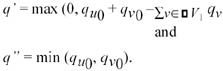
For subsets V′ and V′′ of V, we denote by [V′, V′′]_H the (possibly empty) set of edges of H with one end in V′ and the other in V′′. An edge cut of H is a nonempty subset of E of the form [V′, V− V′]_H where V′ is a proper subset of V. If H is a bipartite connected graph with at least one edge, then there exists a bipartition {V₁, V₂} of V such that the edge set E of H coincides with the edge cut [V₁, V₂]_H; then the sets V₁ and V₂ are called the sides of H. A bond of H is a minimal (with respect to set-inclusion) edge cut of H. (Note that every edge cut of H is the disjoint union of bonds of H.) An edge e of H is a cut edge (or a "bridge") if {e} is a bond of H. A bond F of a bipartite graph H is simple (Malvestuto, 1993) or "bipartite" (Kao, 1997) if, for each connected component H′ of H−F, F is incident to at most one side of H′ (see Figure 3).

Figure 3: A Simple Bond of a Bipartite Graph

A mixed graph is a generalization of an ordinary graph. A mixed graph is a pair H = (V, E ∪ E) where E is a collection of subsets of V of cardinality 1 or 2, and E is a set of ordered pairs of elements of V. The elements of E are called undirected edges of H, and the elements of are called directed edges of H. If the set of undirected edges of H is empty, then H is called a digraph. A directed path in H from vertex u to vertex u′ is a sequence (v₁,…, v_k) of distinct vertices such that u = v₁, u′ = v_k and for all h < k, {v_h, v_h+1} is in E or <v_h, v_h+1> is in. Two vertices u and u′ are strongly connected if there exist a directed path from u to u′ and a directed path from u′ to u. A mixed graph is strongly connected if every two vertices are strongly connected. The strongly connected components of H are the subgraphs of H induced by its maximal sets of pairwise strongly connected vertices. The cross-component edges of H are the directed edges joining two strongly connected components of H.

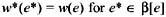
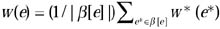
A network N is a digraph (V,E ) with two distinguished vertices, called the source and the sink of N respectively, where each directed edge e has associated to it a nonnegative quantity (possibly, +∞), which is called the capacity of e and denoted by c(e). Let s and t be the source and the sink of N, respectively. A flow in N is a real-valued function φ defined on such that

and

the summations being extended over all v such that <v, u> ∈ E and <u, v> ∈ E, respectively. A maximum flow in N is a flow in N that maximizes the quantity

the summation being extended over all v such that <s, v> ∈ E. Maximum flows in N can be computed in O(|V|³) time.

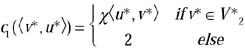
Example 4: Consider the network N shown in Figure 4.

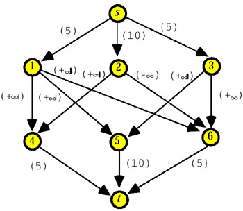
Figure 4

A maximum flow in N is shown in Figure 5.

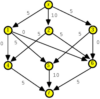
Figure 5

Testing Invariance

Let Q be a graphical query set, and let (H, q) be the answer map of Q. Without loss of generality, in what follows we assume that H is a connected graph with m edges and n vertices. We separately discuss the problem of testing the sum expression Σe ∈ F x(e) for D-invariance in the cases

The Case

We saw that deciding if the sum expression Σe ∈ F x(e) is an -invariant of (H, q) is equivalent to testing the consistency of equation system (3). We now show that this test can be carried out in linear time (Malvestuto & Moscarini, 1999). Since the rank of the incidence matrix of H is equal to n−1 if H is bipartite, and is equal to n otherwise, equation system (3) has at most ∞¹ solutions and can be transformed to an equivalent system Λ of m−n+1 linear equations in one unknown, denoted by λ. It consists of choosing an arbitrary vertex r of H, and performing a depth-first search (DFS) traversal of H with start-vertex r. During the traversal of H, each vertex v, when v is first visited, will be labeled by a linear expression ∊_v(λ) in λ and, for each edge not in the traversal tree of H, a linear equation in λ is added to Λ as is stated by the following algorithm whose output variable inv is True if and only if the sum expression Σe ∈ F x(e) is an -invariant of (H, q).

Algorithm -INVARIANCE

Input: A connected graph H, the incidence vector f of F, and a vertex r of H.

Step 1. inv := False; ∊_r(λ) := λ; Λ := Ø.

Step 2. Start a DFS traversal of H at vertex r. During the traversal of H, when vertex v is reached using edge e, then

Step 3. Test Λ for consistency. If Λ turns out to be consistent, then set inv := True.

It is clear that equation system (3) is equivalent to equation system Λ. Moreover, an equation in Λ of the form ∊u(λ) + ∊_v(λ) = f(e) can have no solutions (i.e., the equation is impossible), one solution (the equation is determined), or ∞ solutions (the equation is an identity), and an equation in of the form ∊_v(λ) = f(e) has always one solution. Note that an equation in Λ is determined if and only if it corresponds to a non-tree edge of H whose addition to the traversal tree creates an odd cycle. Since Λ is consistent if and only if no equation in Λ is impossible and the determined equations in Λ (if any) have all the same solution, it is easy during the traversal of H to check the consistency of Λ so that one can decide in linear time whether equation system Λ and, hence, equation system (3) is consistent and, if this is the case and λ_o is a solution of equation system Λ, one can determine a solution y of equation system (3) by taking y_v = ∊_v(λ_o).

Example 5: Consider again the query set Q = {Q₁, Q₂, Q₃} of Example 3, whose answer map is shown in Figure 2, and assume that D =. Suppose that F = {e₁, e₃}. Using algorithm -INVARIANCE, we can label the vertices as shown in Figure 6 (we are assuming that the DFS traversal starts at vertex 1 and reaches vertices 2 and 3 using edges e₂ and e₃).

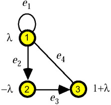
Figure 6

Accordingly, the equation system Λ is the pair of the following two equations corresponding to e₁ and e₃ respectively:

and turns out to be inconsistent. Therefore, we can conclude that the sum expression Σe ∈ F x(e) is not an -invariant of (H, q).

Using algorithm -INVARIANCE, one can prove that, if H is bipartite, then the sum expression Σe ∈ F x(e) is an -invariant of (H, q) if and only if F is the disjoint union of simple bonds (Malvestuto, 1993; Kao, 1997); as a consequence, if the target-query is an elementary query, that is, F = {e} for some edge e of H, then Q belongs to the closure of Q if and only if e is a cut edge of H.

The Case

We now prove that the procedure for deciding if the sum expression Σe ∈ F x(e) is an -invariant of (H, q) can be implemented in O(n³) time using network computation. We distinguish two cases depending on whether H is or is not bipartite.

Assume that H = (V, E) is a bipartite graph with sides V₁ and V₂. Let Net(H, q) be the network (V ∪ {s, t}) with

where the capacities of the directed edges of Net(H, q) are defined as follows

Gusfield (1988) proved that:

1. The solutions of the constraint system associated with Q coincide with the restrictions to E of maximum flows in Net(H, q).

2. Given a maximum flow φ in Net(H, q), let H(φ) be the mixed graph obtained from H by directing each edge {u, v}, u ∈ V₁, and v ∈ V₂, with φ(<u, v>) = 0 from V₁ to V₂; then the set of cross-component edges of H(φ) equals kernel(H).

Therefore, the following algorithm correctly decides if the sum expression Σe ∈ F x(e) is an -invariant of (H, q).

Step 1. Construct the network Net(H, q) and find a maximum flow φ in Net(H, q).

Step 2. Let w be the restriction of φ to E. Construct the mixed graph H(φ) obtained from H by directing from V₁ to V₂ each edge {u, v}, u ∈ V₁, and v ∈ V₂, with j(<u, v>) = 0.

Step 3. Set kernel(H) to the set of cross-component edges of H(w).

Step 4. For each connected component H′ = (V′, E′) of the graph H−kernel(H) with F ∩ E′ ≠ Ø, apply algorithm -INVARIANCE with input H′ and the incidence vector of F ∩ E′. If each time the algorithm terminates with inv = True, then and only then conclude that the sum expression Σe ∈ F x(e) is an -invariant of (H, q).

Since a maximum flow in Net(H, q) can be computed in O(n³) time, algorithm -INVARIANCE can be implemented in O(n³) time.

Example 6: Let Q = {Q₁, Q₂, Q₃, Q₄, Q₅, Q₆} be a set of additive queries with values in , whose answer map is shown in Figure 7.

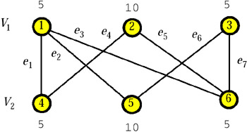
Figure 7

Then, Net(H, q) is the network of Figure 4 and a maximum flow in in Net(H, q) is shown in Figure 5. The mixed graph H(φ) is shown in Figure 8.

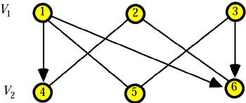
Figure 8

The cross-component edges of H(φ) are <1, 4>, <1, 6>, and <3, 6>. Therefore, kernel(H) is formed by the three edges e₁, e₃, and e₇. Of course, the elementary query corresponding to each edge in kernel(H) belongs to the closure of Q. The graph H−kernel(H) is shown in Figure 9.

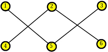
Figure 9

Here, each edge is a cut edge of a bipartite graph and, hence, the corresponding elementary query belongs to the closure of Q. To sum up, every elementary query (and, hence, the target-query) belongs to the closure of Q.

We now discuss the case that H is not bipartite. We associate with H a bipartite, connected graph H* = (V*, E*) which contains 2n vertices and 2m−l edges, where l is the number of self-loops of H. The graph H* is constructed as follows. Let G be a bipartite partial graph of H obtained from a spanning tree of H by adding the nontree edges that create even cycles. Let V′ be a "copy" of V, that is, V′ ∩ V = Ø and |V′| = |V|. If v is a vertex of H, then by v′ we denote the copy of v; moreover, if e = {u, v} is a link of H, then by e′ we denote the set {u′, v′}. The vertex set V* of H* is taken to be the union of V and V′, that is, V* = V ∪ V′. The edge set E* of H* is taken to be

where β[e] is defined as follows:

• if e is an edge of G, then b[e] = {e, e′};

• if e = {u, v} is a link of H but not an edge of G, then b[e] = {{u, v′}, {u′, v}};

• if e is a self-loop of H, say {v}, then β[e] = {{v, v′}}.

Note that since H is a nonbipartite, connected graph, H* is bipartite and connected. Furthermore, if V₁ and V₂ are the sides of G, then the sides of H* are V*₁ = V₁ ∪ V₂′ and V*₂ = V₁ ∪ V₂, where V_i′ = {v′: v ∈ V_i}, i = 1, 2. For each v in V set q*_v := q_v, and for each v′ in V′, set q*_v′ := q_v.

Example 7: Consider again the query set Q = {Q₁, Q₂, Q₃} of Example 3, whose answer map was shown in Figure 2, and assume that . By choosing as G the graph shown in Figure 10, we obtain the bipartite vertex-weighted graph H* shown in Figure 11.

Figure 10

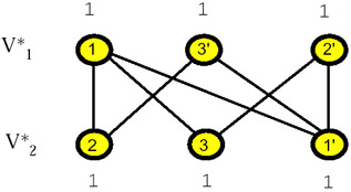
Figure 11

Let Γ* be the system of linear constraints given by the equation system

where H* is the incidence matrix of H*, with the addition of the nonnegativity constraints

Malvestuto & Mezzini (2000) proved that:

1. If w is a solution of G, then the vector w* with

   

   is a solution of Γ*, and if w* is a solution of Γ*, then the vector w with

   

   is a solution of Γ.

2. kernel(H) = {e ∈ E: β[e] ⊆ kernel(H*)}.

By combining these results with Gusfield's results, one has also in the case that H is not bipartite; the procedure for testing invariance can be implemented in O(n³) time.

Example 7 (continued): The constraint system Γ* reads

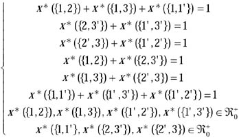
The general solution of Γ* is

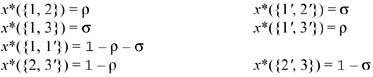
where ρ an σ are bounded as shown in Figure 12:

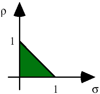
Figure 12

We now show how kernel(H) can be graphically obtained. Figure 13 shows Net(H*, q*)and Figure 14 shows a maximum flow φ* in Net(H*, q*).

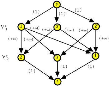
Figure 13

Figure 14

The mixed graph H*(φ*) coincides with H* which is strongly connected. So, kernel(H*) is empty, and kernel(H) is empty too.

Computing the Feasibility Range

Assume that the target-query Q is an elementary query and that e is the edge corresponding to Q. Let q′ and q′′ be the tightest lower and upper bounds on the value of Q. Here we show how q′ and q′′ can be efficiently computed in the case .

We distinguish two cases depending on whether H is or is not bipartite, and we shall solve the problem of computing q′ and q′′ with the method given by Gusfield (1988) in the former case, and by Malvestuto & Mezzini (2002) in the latter case.

Assume that H is a bipartite graph with sides V₁ and V₂, and let e = {u_o, v_o} with u_o ∈ V₁ and v_o ∈ V₂. We first find a maximum flow φ in the network Net(H, q). Given φ, let us construct the digraph N with vertex set V and directed-edge set

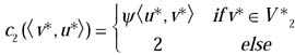
For each directed edge <u, v> of N, take its capacity to be

where M is a finite number larger than the largest q_v for v in V₁. Let N₁ be the network with underlying digraph N having source u_o and sink v_o, and let φ₁ be a maximum flow in N₁. Analogously, let N₂ be the network with underlying digraph N having source v_o and sink u_o, and let φ₂ be a maximum flow in N₂. If Φ₁(u_o → v_o) and Φ₂(v_o → u_o) are respectively the values of φ₁ and φ₂, then q′ and q′′ are given by

and

Moreover, if H is a complete bipartite graph, then α₁ and α₂ are simply given by

Therefore, the tightest lower and upper bounds on the value of Q can be found in O(n³) time.

Example 8: Let Q = {Q₁, Q₂, Q₃, Q₄, Q₅, Q₆} be a set of additive queries with values in, whose answer map is shown in Figure 15.

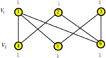
Figure 15

Figure 16 shows a maximum flow φ in Net(H, q).

Figure 16

Suppose that the target-query Q is the query corresponding to the edge {1, 6}. In order to compute the tightest lower bound q′ and the tightest upper bound q′′ on the value of Q, we construct the digraph N, which is shown in Figure 17.

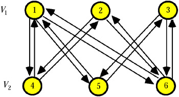
Figure 17

Next, consider the network N₁ on N with source vertex 1 and sink vertex 6, and with capacities defined as follows:

A maximum flow φ₁ in N₁ is shown in Figure 18.

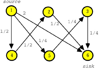
Figure 18

The value of φ₁ is Φ₁(1 → 6) = 11/4 so that, by formula (5), one obtains q′ = max (0, φ(<1, 6>) − Φ₁(1 → 6) + 2) = max (0, 1/4 − 11/4 + 2) = 0.

Consider now the network N₂ which differs from N₁ only in that the source and the sink are vertices 6 and 1, respectively. A maximum flow φ₂ in N₂ is shown in Figure 19.

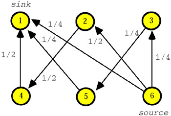
Figure 19

The value of φ₂ is Φ₂(6 → 1) = 1 so that, by formula (6), one obtains

Consider now the case that H is not bipartite. Let H* be a bipartite transform of H and Γ* the constraint system as stated in the "Graphs and Networks" subsection above. Let β[e] be the image of e in H*. If e is a self-loop and β[e] = {e*}, then the tightest lower and upper bounds on the value of Q are given by

so that q′ and q′′ can be determined in O(n³) time using Gusfield's method applied to H*. Otherwise, that is, if e is a link and β[e] = {e*₁, e*₂}, let

Then, the tightest lower and upper bounds on the value of Q are given by

With an example we show that α₁ and α₂ (and hence q′ and q′′) can be computed in O(n³) time.

Example 7 (continued): Suppose that the target-query Q is the elementary query corresponding to the self-loop {1}. By formula (5), the tightest lower and upper bounds on the value of Q are given by

To compute them, we can proceed as in Example 8 when min x({1, 6}) and max x({1, 6}) were computed. So, one has

Suppose now that the target-query Q is the elementary query corresponding to the edge {2, 3}. The tightest lower and upper bounds on the value of Q are respectively given by formula (7) where

We show how to compute α₁ and α₂ in cubic time. For both of them, we make use of a maximum flow in Net(H*, q*). Let ϕ be the maximum flow in Net(H*, q*) shown in Figure 20.

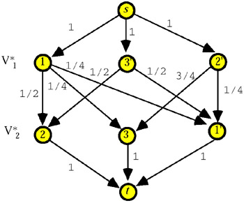
Figure 20

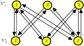
Figure 21

Let us begin with the computation of α₁. First of all, we compute min x*({2, 3'}) subject to Γ* using the above procedure for bipartite graphs. More precisely, we construct the network N₁ on the digraph with source vertex 3' and sink vertex 2, and with capacities defined as follows:

A maximum flow φ₁ in N₁ is shown in Figure 22.

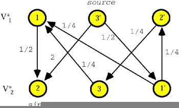
Figure 22

The value of φ₁ is Φ₁(3′ → 2) = 5/2 so that, by formula (5), one has min x*({2, 3′}) = max (0, φ(<3′, 2>) − Φ₁(3′ → 2) + 2) = max (0, 1/2 − 5/ 2 + 2) = 0.

After computing min x*({2, 3′}) (= 0), we calculate α₁ as min x*({2, 3′}) plus the quantity

To achieve this, let (H*−{2, 3′}, q*1) be the vertex-weighted graph obtained from (H*, q*) by deleting the edge {2, 3′} and subtracting min x*({2, 3′}) (= 0) from the weights of the endpoints of the edge {2, 3′} (see Figure 23).

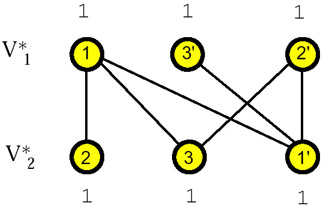
Figure 23

Then, the quantity

equals min x*({2′, 3}) in (H*–{2, 3′}, q*1), which is found with the same technique employed to find min x*({2, 3′}) in (H*, q*). That is, we first find a maximum flow χ in Net(H*−{2, 3′}, q*1). Let χ be the maximum flow in Net(H*−{2, 3′}) shown in Figure 24.

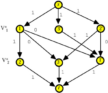
Figure 24

Next, let D be the digraph (see Figure 25) with vertex set V* and directed-edge set

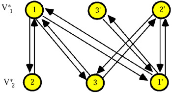
Figure 25

Then, we construct the network M1 on D with source vertex 2′ and sink vertex 3, and capacities defined as follows:

and compute a maximum flow in M₁. Let χ₁ be the maximum flow in M₁ shown in Figure 26.

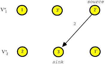
Figure 26

The value of χ₁ is X₁(2′ → 3) = 2 so that, by formula (5), one has that min x*({2′, 3}) in (H*−{2, 3′}, q*1) is equal to

Finally, we obtain

and, by formula (7),

As to α₂, we proceed as follows. First of all, we compute max x*({2, 3′}) subject to Γ*. To this end, we construct the network N₂ which differs from N₁ only in the source and the sink which are not set to vertex 3′ and vertex 2, respectively. A maximum flow φ₂ in N₂ is shown in Figure 27.

Figure 27

The value of φ₂ is Φ₂(2 → 3′) = 1 so that, by formula (6), one has

After computing max x*({2, 3′}), we calculate α₂ as max x*({2, 3′}) plus the quantity

To achieve this, let (H−{2, 3′}, q*2) be the vertex-weighted graph obtained from H* by deleting edge {2, 3′} and subtracting max x*({2, 3′}) (= 1) from the weights of the endpoints of edge {2, 3′} (see Figure 28).

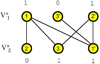
Figure 28

Then, the quantity

equals max x*({2′, 3}) in (H*−{2, 3′}, q*2), which is found with the same technique employed to find max x*({2, 3′}) in (H*, q*). That is, we first find a maximum flow in Net(H*−{2, 3′}, q*2). Let Ψ the maximum flow in Net(H*−{2, 3′}, q*2) shown in Figure 29.

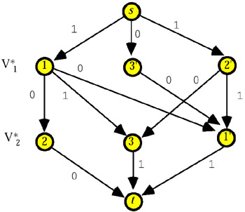
Figure 29

Then, we construct the network M₂ on D with source vertex 3 and sink vertex 2′, and capacities defined as follows:

and compute a maximum flow in M₂. Let ψ₂ be the maximum flow in M₂ shown in Figure 30.

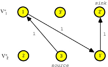
Figure 30

The value of ψ₂ is Ψ₂(3 → 2′) = 1 so that, by formula (6), one has max x*({3, 2′}) = Ψ₂(3 → 2′) = 1.

Finally, we obtain

and

Before closing this section, we note that the existence of an efficient membership test, and of an efficient procedure for computing the tightest lower and upper bounds on the value of an elementary query in the case D = Z₀⁺, is an open problem; however, if H is bipartite, then the total unimodularity of its incidence matrix allows us to apply the procedures above stated for the case .