8.5 Data Access Methods
|
| < Day Day Up > |
|
This section on data access methods will cover a lot of ground. General areas covered are as follows:
-
Tables, Indexes, and Clusters. There are numerous ways to access data objects.
-
Joins. The Optimizer has specific methods of joining tables, largely determined by table sizes.
-
Sorting. The Optmizer sorts SQL statement output in various ways.
-
Special Cases. Concatenation, IN list operators, and UNION operators warrant special mention.
-
Hints. Hints allow overriding of a path of execution selected by the Optimizer for an SQL statement.
8.5.1 Accessing Tables and Indexes
In this section we examine the different ways in which the Optimizer accesses tables and indexes. Tables can be full scanned, sampled, or scanned by a ROWID passed from an index. There are a multitude of ways in which indexes can be accessed and many ways in which index scanning can be affected. There are some important things to note about indexes:
-
An index will occupy a small percentage of the physical space used by a table. Thus searching through an index either precisely or fully is usually much faster than scanning a table.
-
Reading an index to find a ROWID pointer to a table can speed up access to table rows phenomenally.
-
Sometimes tables do not have to be read at all where an index contains all the retrieved column data.
Full Table Scans
Reading Many Blocks at Once
A full table scan can be speeded up by reading multiple blocks for each read. This can be done using the DB_FILE_MULTIBLOCK _READ_COUNT parameter. This parameter is usually set between 4 and 16, typically 4, 8, or 16. The default value is 8. You might want to consider setting it to 4 or less for OLTP systems and 16 or higher for data warehouses.
| Tip | I set the value of DB_FILE_MULTIBLOCK_READ_COUNT on my Win2K server to various values between 1 and 128 and had no problems. This parameter is not restricted to specific values. |
A full table scan may result if the number of blocks occupied by a table is less than DB_FILE_MULTIBLOCK_READ_COUNT. Please note the emphasis on the term "may result"; it is not an absolute. The Optimizer is very sophisticated in the current version of Oracle Database and is unlikely to conclude that a full table scan is faster than an index plus ROWID pointer table read, especially where a unique index hit is involved on a large table.
Small Static Tables
For a small, static table a full table scan can often be the most efficient access method. A static table is obviously not changed and thus there are never deletions. In many cases an index unique hit will be preferred by the Optimizer since the cost will be lower, particularly in mutable joins. Let's examine small static tables. Let's start by showing the row and block counts from the table statistics in the Accounts schema.
SELECT table_name, num_rows, blocks FROM user_tables ORDER BY 1; TABLE_NAME NUM_ROWS BLOCKS ---------------- -------- ------ CASHBOOK 188185 1517 CASHBOOKLINE 188185 616 CATEGORY 13 1 COA 55 1 CUSTOMER 2694 60 GENERALLEDGER 752741 3244 ORDERS 172304 734 ORDERSLINE 540827 1713 PERIOD 72 1 PERIODSUM 221 1 POSTING 8 1 STOCK 118 4 STOCKMOVEMENT 570175 2333 STOCKSOURCE 12083 30 SUBTYPE 4 1 SUPPLIER 3874 85 TRANSACTIONS 188185 1231 TRANSACTIONSLINE 570175 1811 TYPE 6 1
Looking at the block space occupied by the Accounts schema tables we can see that the COA and Type tables occupy a single block. First of all let's show the relative costs between a unique index hit and full table scan on the Type table. The Type table is very small and occupies considerably less space than the single block it uses.
A full table scan on the Type table has a cost of 2.
EXPLAIN PLAN SET statement_id='TEST' FOR SELECT * FROM type; Query Cost Rows Bytes ----------------------------------- ---- ------ ------- SELECT STATEMENT on 2 6 48 TABLE ACCESS FULL on TYPE 2 6 48
The following query will access both the index and the table. Accessing a single row reads 1/6th of the bytes and the cost is halved.
EXPLAIN PLAN SET statement_id='TEST' FOR SELECT * FROM type WHERE type = 'A'; Query Cost Rows Bytes ----------------------------------- ---- ------ ------- SELECT STATEMENT on 1 1 8 TABLE ACCESS BY INDEX ROWID on TYPE 1 1 8 INDEX UNIQUE SCAN on XPK_TYPE 6
Even a full scan on just the index still has half the cost. The full scan of the index also reads fewer bytes than the unique index scan.
EXPLAIN PLAN SET statement_id='TEST' FOR SELECT type FROM type; Query Cost Rows Bytes ----------------------------------- ---- ------ ------- SELECT STATEMENT on 1 6 6 INDEX FULL SCAN on XPK_TYPE 1 6 6
Now let's go completely nuts! Let's read the same table a multitude of times within the same query. We can see from the query plan following that even though the table is read many times the Optimizer will still assess the cost as 1. There are a multitude of unique index hits, even though the COA table is read in its entirety. We could run timing tests. Results do not imply that the Optimizer is giving us the fastest option.
EXPLAIN PLAN SET statement_id='TEST' FOR SELECT * FROM orders WHERE type IN (SELECT type FROM type WHERE type IN (SELECT type FROM type WHERE type IN (SELECT type FROM type WHERE type IN (SELECT type FROM type WHERE type IN (SELECT type FROM type WHERE type IN (SELECT type FROM type WHERE type IN (SELECT type FROM type WHERE type IN (SELECT type FROM type WHERE type IN (SELECT type FROM type WHERE type IN (SELECT type FROM type)))))))))); Query Cost Rows Bytes ----------------------------------- ---- ------ ------- SELECT STATEMENT on 2 55 1870 NESTED LOOPS on 2 55 1870 NESTED LOOPS on 2 55 1815 NESTED LOOPS on 2 55 1760 NESTED LOOPS on 2 55 1705 NESTED LOOPS on 2 55 1650 NESTED LOOPS on 2 55 1595 NESTED LOOPS on 2 55 1540 NESTED LOOPS on 2 55 1485 NESTED LOOPS on 2 55 1430 NESTED LOOPS on 2 55 1375 TABLE ACCESS FULL on COA 2 55 1320 INDEX UNIQUE SCAN on XPK_TYPE 1 1 INDEX UNIQUE SCAN on XPK_TYPE 1 1 INDEX UNIQUE SCAN on XPK_TYPE 1 1 INDEX UNIQUE SCAN on XPK_TYPE 1 1 INDEX UNIQUE SCAN on XPK_TYPE 1 1 INDEX UNIQUE SCAN on XPK_TYPE 1 1 INDEX UNIQUE SCAN on XPK_TYPE 1 1 INDEX UNIQUE SCAN on XPK_TYPE 1 1 INDEX UNIQUE SCAN on XPK_TYPE 1 1 INDEX UNIQUE SCAN on XPK_TYPE 1 1
Now we will attempt something a little more sensible by running the EXPLAIN PLAN command for a join accessing the COA table four times and then time testing that query. There are four unique scans on the COA table.
EXPLAIN PLAN SET statement_id='TEST' FOR SELECT t.*, cb.* FROM transactions t JOIN cashbook cb ON(t.transaction_id = cb.transaction_id) WHERE t.drcoa# IN (SELECT coa# FROM coa) AND t.crcoa# IN (SELECT coa# FROM coa) AND cb.drcoa# IN (SELECT coa# FROM coa) AND cb.crcoa# IN (SELECT coa# FROM coa); Query Cost Rows Bytes ----------------------------------- ---- ------ ------- 1. SELECT STATEMENT on 7036 188185 22394015 2. NESTED LOOPS on 7036 188185 22394015 3. NESTED LOOPS on 7036 188185 21264905 4. NESTED LOOPS on 7036 188185 20135795 5. NESTED LOOPS on 7036 188185 19006685 6. MERGE JOIN on 7036 188185 17877575 7. TABLE ACCESS BY INDEX ROWID on CASH 826 188185 9973805 8. INDEX FULL SCAN on XFK_CB_TRANS 26 188185 7. SORT JOIN on 6210 188185 7903770 8. TABLE ACCESS FULL on TRANSACTIONS 297 188185 7903770 6. INDEX UNIQUE SCAN on XPK_COA 1 6 5. INDEX UNIQUE SCAN on XPK_COA 1 6 4. INDEX UNIQUE SCAN on XPK_COA 1 6 3. INDEX UNIQUE SCAN on XPK_COA 1 6
In the next query plan I have suggested a full table scan to the Optimizer on the COA table with an overriding hint. The cost has a 20% increase.
EXPLAIN PLAN SET statement_id='TEST' FOR SELECT t.*, cb.* FROM transactions t JOIN cashbook cb ON(t.transaction_id = cb.transaction_id) WHERE t.drcoa# IN (SELECT /*+ FULL(coa) */ coa# FROM coa) AND t.crcoa# IN (SELECT /*+ FULL(coa) */ coa# FROM coa) AND cb.drcoa# IN (SELECT /*+ FULL(coa) */ coa# FROM coa) AND cb.crcoa# IN (SELECT /*+ FULL(coa) */ coa# FROM coa); Query Cost Rows Bytes ----------------------------------- ---- ------ ------- 1. SELECT STATEMENT on 8240 188185 22394015 2. HASH JOIN on 8240 188185 22394015 3. TABLE ACCESS FULL on COA 2 55 330 3. HASH JOIN on 7916 188185 21264905 4. TABLE ACCESS FULL on COA 2 55 330 4. HASH JOIN on 7607 188185 20135795 5. TABLE ACCESS FULL on COA 2 55 330 5. HASH JOIN on 7314 188185 19006685 6. TABLE ACCESS FULL on COA 2 55 330 6. MERGE JOIN on 7036 188185 17877575 7. TABLE ACCESS BY INDEX ROWID on CASH 826 188185 9973805 8. INDEX FULL SCAN on XFK_CB_TRANS 26 188185 7. SORT JOIN on 6210 188185 7903770 8. TABLE ACCESS FULL on TRANSACTIONS 297 188185 7903770
Now let's do some timing tests. Even though query plan costs are higher for full table scans the timing tests following show that the overriding hint full table scans are actually almost twice as fast. Perhaps the Optimizer should have been intelligent enough in the case of this query to force all the COA tables to be read as full table scans.
SQL> SELECT COUNT(*) FROM(SELECT t.*, cb.* 2 FROM transactions t JOIN cashbook cb 3 ON(t.transaction_id = cb.transaction_id) 4 WHERE t.drcoa# IN (SELECT coa# FROM coa) 5 AND t.crcoa# IN (SELECT coa# FROM coa) 6 AND cb.drcoa# IN (SELECT coa# FROM coa) 7 AND cb.crcoa# IN (SELECT coa# FROM coa)); COUNT(*) ----------- 188185 Elapsed: 00:00:11.08 SQL> SELECT COUNT(*) FROM(SELECT t.*, cb.* 2 FROM transactions t JOIN cashbook cb 3 ON(t.transaction_id = cb.transaction_id) 4 WHERE t.drcoa# IN (SELECT /*+ FULL(coa) */ coa# FROM coa) 5 AND t.crcoa# IN (SELECT /*+ FULL(coa) */ coa# FROM coa) 6 AND cb.drcoa# IN (SELECT /*+ FULL(coa) */ coa# FROM coa) 7 AND cb.crcoa# IN (SELECT /*+ FULL(coa) */ coa# FROM coa)); COUNT(*) ----------- 188185 Elapsed: 00:00:07.07
Reading Most of the Rows
Reading a large percentage of the rows in a table can cause the Optimizer to perform a full table scan. This percentage is often stated as being anywhere between 5% and 25%. The following example against the Stock table switches from an index range scan to a full table scan at 30 rows: 30 out of 118 rows which is about 25%. Note how the cost of the two queries is the same.
EXPLAIN PLAN SET statement_id='TEST' FOR SELECT * FROM stock WHERE stock_id <= 29; Query Cost Rows Bytes ----------------------------------- ---- ------ ------- SELECT STATEMENT on 2 29 6757 TABLE ACCESS BY INDEX ROWID on STOCK 2 29 6757 INDEX RANGE SCAN on XPK_STOCK 1 29 EXPLAIN PLAN SET statement_id='TEST' FOR SELECT * FROM stock WHERE stock_id <= 30; Query Cost Rows Bytes ----------------------------------- ---- ------ ------- SELECT STATEMENT on 2 30 6990 TABLE ACCESS FULL on STOCK 2 30 6990
Reading Deleted Rows
A full table scan simply reads the entire table. The biggest potential problem with a full table scan is that all blocks ever used by the table will be read, not just all the rows in the table. What does this mean? The high water mark bears mentioning. What is the high water mark? The high water mark for a table is the largest number of blocks ever allocated to a table. As rows are added to a table the high water mark (number of blocks used) increases. When data is deleted from that table using the DELETE command the high water mark does not decrease. Only the TRUNCATE command or recreating the table with the CREATE TABLE command will decrease the high water mark.
If a table that had many rows added is then deleted from completely and full table scanned, what will be the result? All the blocks deleted from will be read even though the table has no rows at all. The following example proves this. Full table scans on very large tables subject to large amounts of deletion can cause serious performance problems. Let's look at deleting from tables. The first query plan reads all data from the OrdersLine table. Note the cost, rows, and bytes read.
EXPLAIN PLAN SET statement_id='TEST' FOR SELECT * FROM ordersline; Query Cost Rows Bytes ----------------------------------- ---- ------ ------- SELECT STATEMENT on 765 997903 15966448 TABLE ACCESS FULL on ORDERSLINE 765 997903 15966448
Now I delete all the rows from the table and run the EXPLAIN PLAN command again. The rows and bytes values have decreased dramatically but the cost is identical regardless of all the rows being deleted. Additionally I have updated statistics. I am copying my OrdersLine table to a temporary table so that I can retrieve the OrdersLine table rows.
DROP TABLE tmp; CREATE TABLE tmp AS SELECT * FROM ordersline; DELETE FROM ordersline; COMMIT; ANALYZE TABLE ordersline COMPUTE STATISTICS; EXPLAIN PLAN SET statement_id='TEST' FOR SELECT * FROM ordersline; Query Cost Rows Bytes ----------------------------------- ---- ------ ------- SELECT STATEMENT on 765 1 52 TABLE ACCESS FULL on ORDERSLINE 765 1 52
Now I will TRUNCATE the table and run my EXPLAIN PLAN command again. I must not forget to compute the statistics again otherwise the Optimizer will use previously calculated statistics, namely statistics showing almost a million rows in the OrdersLine table, when it is now empty. The query plan is drastically different now with the cost much reduced.
TRUNCATE TABLE ordersline; ANALYZE TABLE ordersline COMPUTE STATISTICS; EXPLAIN PLAN SET statement_id='TEST' FOR SELECT * FROM ordersline; Query Cost Rows Bytes ----------------------------------- ---- ------ ------- SELECT STATEMENT on 2 1 52 TABLE ACCESS FULL on ORDERSLINE 2 1 52
A serious potential problem with full table scans is scanning up to the high water mark to include blocks which once contained rows that have now been deleted.
Now let's retrieve the OrdersLine table.
INSERT INTO ordersline SELECT * FROM tmp; COMMIT;
So what can we conclude about full table scans. In short they are usually best avoided. In rare circumstances they can be faster than index scans, particularly for small static tables. A full table scan will result when no index is available or when an index is missed accidentally by, for instance, including a function on a column in a WHERE clause where no matching function-based index exists.
Parallel Full Table Scans
Let's try scanning a large table in parallel. Parallel scans can be induced on full table scans by using the PARALLEL hint or by setting the PARALLEL attribute when creating or altering a table. Let's look at changing a table. The GeneralLedger table is the largest table in the Accounts schema and is thus the most appropriate for parallel processing. Also I have a dual CPU machine. I do not however have Oracle Partitioning at this point. Oracle Partitioning is covered in Part III.
ALTER TABLE generalledger PARALLEL 2;
The degree of parallelism can be verified by using the following query.
SELECT table_name, degree FROM USER_TABLES:
Now let's look at a query plan. Note I am using an adjusted PLAN_TABLE query including the OTHER_TAG column (see Appendix B).
EXPLAIN PLAN SET statement_id='TEST' FOR SELECT * FROM generalledger; Query Cost Rows ----------------------------------------- ---- ------ 1. SELECT STATEMENT on 195 752740 2. TABLE ACCESS FULL on GENERALLEDGER PARALLEL_TO_SERIAL 195 752740
Now let's remove the parallelism from the GeneralLedger table again.
ALTER TABLE generalledger NOPARALLEL;
Now let's check the query plan again. There is no difference in cost.
EXPLAIN PLAN SET statement_id='TEST' FOR SELECT * FROM generalledger; Query Cost Rows Bytes ----------------------------------- ---- ------ ------- 1. SELECT STATEMENT on 195 752740 19571240 2. TABLE ACCESS FULL on GENERALLEDGER 195 752740 19571240
Let's do some timing tests. Once again we set the degree of parallelism on the table to 2.
ALTER TABLE generalledger PARALLEL 2; SQL> SELECT COUNT(*) FROM(SELECT /*+ FULL(gl) */ * FROM generalledger gl); COUNT(*) ----------- 752741 Elapsed: 00:00:05.06
Now increase the degree of parallelism on the table.
ALTER TABLE generalledger PARALLEL 4;
The time taken is slightly less with the degree of parallelism increased.
SQL> SELECT COUNT(*) FROM(SELECT /*+ FULL(gl) */ * FROM generalledger gl); COUNT(*) ----------- 752741 Elapsed: 00:00:05.02
Lastly, remove parallelism from the table altogether. The elapsed time is much faster without parallelism as shown in the query plan following. Parallel queries should only be used on very large row sets. OLTP databases should avoid large row sets and therefore parallelism is most appropriate to large data warehouses and not OLTP databases. Parallelism in general applies to full table scans, fast full index scans, and on disk sorting, in other words physical I/O activity, and preferably using Oracle Partitioning.
ALTER TABLE generalledger NOPARALLEL; SQL> SELECT COUNT(*) FROM(SELECT /*+ FULL(gl) */ * FROM generalledger gl); COUNT(*) ----------- 752741 Elapsed: 00:00:01.01
Sample Table Scans
A sample scan can be used to sample a percentage of a table either by rows or blocks, useful if you want to examine a small part of a table. The row count is much lower in the second 0.001% sampled query following.
EXPLAIN PLAN SET statement_id='TEST' FOR SELECT * FROM generalledger; Query Cost Rows Bytes ----------------------------------- ---- ------ ------- SELECT STATEMENT on 715 1068929 24585367 TABLE ACCESS FULL on GENERALLEDGER 715 1068929 24585367 EXPLAIN PLAN SET statement_id='TEST' FOR SELECT * FROM generalledger SAMPLE(0.001); Query Cost Rows Bytes ----------------------------------- ---- ------ ------- SELECT STATEMENT on 715 11 253 TABLE ACCESS SAMPLE on GENERALLEDGER 715 11 253
| Note | Oracle Database 10 Grid A seeding value option has been added to the sample clause to allow Oracle Database to attempt to return the same sample of rows or blocks across different executions as shown in the syntax following. |
SELECT ¼ SAMPLE( % ) [ SEED n ];
ROWID Scans
A ROWID is an Oracle Database internal logical pointer to a row in a table. An index stores index column values plus a ROWID pointing to a row in a table. When an index is read the ROWID found for an index value is used to retrieve that row from the table directly. For a unique index hit at most three block reads are made in the index space and one block read in the table space. An index to table ROWID scan is shown in Figure 8.3.
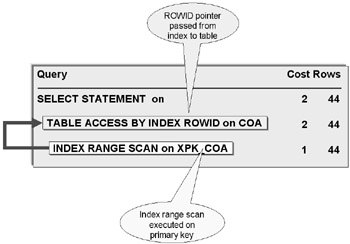
Figure 8.3: Passing a ROWID Pointer from an Index to a Table
EXPLAIN PLAN SET statement_id= 'TEST' FOR SELECT * FROM coa WHERE coa# < '50000';
Index Scans
An index is a subset of a table containing a smaller number of columns. Each row in an index is linked to a table using a ROWID pointer. A ROWID pointer is an Oracle Database internal logical representation based on a datafile, a tablespace, a table, and block. Effectively a ROWID is an address pointer and is the fastest method of access for rows in the Oracle database.
There are numerous different types of index scans:
-
Index Unique Scan. Uses a unique key to return a single ROWID, which in turn finds a single row in a table. A unique scan is an exact row hit on a table and the fastest access for both index and table.
-
Index Range Scan. Scans a range of index values to find a range of ROWID pointers.
-
Reverse Order Index Range Scan. This is an index range scan in descending (reverse) order.
-
-
Index Skip Scan. Allows skipping of the prefix of a composite index and searches the suffix index column values.
-
Index Full Scan. Reads the entire index in the key order of the index.
-
Fast Full Index Scan. Reads an entire index like an index full scan but reads the index in physical block rather than key order. Thus when reading a large percentage of a table without a requirement for sorting a fast full index scan can be much faster than an index full scan.
Tip A fast full index scan is executed in the same manner as that of a full table scan in that it reads data directly from disk and bypasses the buffer cache. As a result a fast full index scan will absolutely include I/O activity and load into the buffer cache but not read the buffer cache.
-
Index Join. This is a join performed by selecting from multiple BTree indexes.
-
Bitmap Join. Joins using bitmap key values, all read from indexes.
-
Let's demonstrate the use of each type of index scan.
Index Unique Scan
A unique scan or exact index hit reads a unique index and finds a single row. Unique scans usually occur with equality comparisons and IN or EXISTS subquery clauses.
EXPLAIN PLAN SET statement_id= 'TEST' FOR SELECT * FROM coa WHERE coa# = '60001'; Query Cost Rows Bytes ----------------------------------- ---- ------ ------- SELECT STATEMENT on 1 1 24 TABLE ACCESS BY INDEX ROWID on COA 1 1 24 INDEX UNIQUE SCAN on XPK_COA 55 EXPLAIN PLAN SET statement_id= 'TEST' FOR SELECT * FROM coa WHERE coa# = '60001' AND type IN (SELECT type FROM type); Query Cost Rows Bytes ----------------------------------- ---- ------ ------- SELECT STATEMENT on 1 1 25 NESTED LOOPS on 1 1 25 TABLE ACCESS BY INDEX ROWID on COA 1 1 24 INDEX UNIQUE SCAN on XPK_COA 55 INDEX UNIQUE SCAN on XPK_TYPE 1 1 EXPLAIN PLAN SET statement_id= 'TEST' FOR SELECT * FROM coa WHERE coa# = '60001' AND EXISTS (SELECT type FROM type WHERE type = coa.type); Query Cost Rows Bytes ----------------------------------- ---- ------ ------- SELECT STATEMENT on 1 1 25 NESTED LOOPS SEMI on 1 1 25 TABLE ACCESS BY INDEX ROWID on COA 1 1 24 INDEX UNIQUE SCAN on XPK_COA 55 INDEX UNIQUE SCAN on XPK_TYPE 6 6
Index Range Scan
Range scans typically occur with range comparisons <, >, <=, >=, and BETWEEN. A range scan is less efficient than a unique scan because an index is traversed and read many times for a group of values rather than up to the three reads required for a unique scan.
EXPLAIN PLAN SET statement_id= 'TEST' FOR SELECT * FROM generalledger WHERE generalledger_id < 10; Query Cost Rows Bytes ----------------------------------- ---- ------ ------- SELECT STATEMENT on 4 1 23 TABLE ACCESS BY INDEX ROWID on GENERALLEDGER 4 1 23 INDEX RANGE SCAN on XPK_GENERALLEDGER 3 1
The next query reads the GeneralLedger table as opposed to the COA table and reads a large percentage of a very large table. The Optimizer switches from an index range scan to a full table scan since most of the table is read.
EXPLAIN PLAN SET statement_id= 'TEST' FOR SELECT * FROM generalledger WHERE generalledger_id > 10; Query Cost Rows Bytes ----------------------------------- ---- ------ ------- SELECT STATEMENT on 715 1068929 24585367 TABLE ACCESS FULL on GENERALLEDGER 715 1068929 24585367
Forcing index use also avoids a range scan but the cost is very much higher than scanning the whole table because an ordered full index scan is used. Suggesting a fast full index scan using the INDEX_FFS hint would probably be faster than a full table scan.
EXPLAIN PLAN SET statement_id='TEST' FOR SELECT /*+ INDEX(generalledger, XPK_GENERALLEDGER) */ * FROM generalledger WHERE coa# < '60001'; Query Cost Rows Bytes ----------------------------------- ---- ------ ------- SELECT STATEMENT on 7052 890774 20487802 TABLE ACCESS BY INDEX ROWID on GENERALLEDGER 7052 890774 20487802 INDEX FULL SCAN on XPK_GENERALLEDGER 2309 1068929
Reverse Order Index Range Scan
A reverse order index range scan is used when rows are sorted in descending order.
EXPLAIN PLAN SET statement_id='TEST' FOR SELECT * FROM generalledger WHERE generalledger_id < 10 ORDER BY 1 DESC; Query Cost Rows Bytes ----------------------------------- ---- ------ ------- SELECT STATEMENT on 4 1 23 TABLE ACCESS BY INDEX ROWID on GENERALLEDGER 4 1 23 INDEX RANGE SCAN DESCENDING on XPK_GENERALLEDGER 3 1
Index Skip Scan
An index skip scan will allow skipping of a prefix column in a composite index and still utilize the index. This assumes that reading that index is faster than scanning the whole table. The Accounts schema does not have an appropriate index to demonstrate an index skip scan so we can create one. The Orders table has a type column set to "S" for "Sales" or "P" for "Purchase". An index skip scan is used when the prefix of a composite index has low cardinality (few values) and the suffix has high cardinality (many different values).
CREATE INDEX xak_o_type_customer ON orders(type, customer_id) COMPUTE STATISTICS;
Now let's find some values.
SELECT * FROM( SELECT type, customer_id, COUNT(customer_id) FROM orders WHERE customer_id IS NOT NULL GROUP BY type, customer_id) WHERE ROWNUM <= 10; T CUSTOMER_ID COUNT(CUSTOMER_ID) - ----------- ------------------ S 1 22 S 2 8 S 3 47 S 4 8 S 5 41 S 6 15 S 7 15 S 8 55 S 9 17 S 10 10
Firstly, use the index as a composite.
EXPLAIN PLAN SET statement_id='TEST' FOR SELECT type, customer_id FROM orders WHERE type = 'S' AND customer_id = 8; Query Cost Rows Bytes ----------------------------------- ---- ------ ------- SELECT STATEMENT on 1 12 36 INDEX RANGE SCAN on XAK_O_TYPE_CUSTOMER 1 12 36
Now remove the type column index prefix from the WHERE clause. The same index is used with an index skip scan, skipping the prefix.
EXPLAIN PLAN SET statement_id='TEST' FOR SELECT type, customer_id FROM orders WHERE customer_id = 8; Query Cost Rows Bytes ----------------------------------- ---- ------ ------- SELECT STATEMENT on 3 24 72 INDEX SKIP SCAN on XAK_O_TYPE_CUSTOMER 3 24 72
Selecting all columns uses a range scan on a different index because the CUSTOMER_ID column has an index. There is a foreign key index on the CUSTOMER_ID column.
EXPLAIN PLAN SET statement_id='TEST' FOR SELECT * FROM orders WHERE customer_id = 8; Query Cost Rows Bytes ----------------------------------- ---- ------ ------- SELECT STATEMENT on 7 24 552 TABLE ACCESS BY INDEX ROWID on ORDERS 7 24 552 INDEX RANGE SCAN on XFK_O_CUSTOMER 1 24
Index Full Scan
A full index scan reads the entire index in key order and not the physical block order of the index. Retrieved columns must be in the index with one non-NULL column, as can be seen in the following two examples. The first example shows a single-column primary key index and the second a multiple-column composite primary key index.
EXPLAIN PLAN SET statement_id='TEST' FOR SELECT stock_id FROM stock; Query Cost Rows Bytes ----------------------------------- ---- ------ ------- SELECT STATEMENT on 1 118 354 INDEX FULL SCAN on XPK_STOCK 1 118 354 EXPLAIN PLAN SET statement_id='TEST' FOR SELECT year, period, coa# FROM periodsum; Query Cost Rows Bytes ----------------------------------- ---- ------ ------- SELECT STATEMENT on 1 45 450 INDEX FULL SCAN on XPK_PERIODSUM 1 45 450
The benefit of a full index scan is a sorted result since the index is scanned in sorted key order. Sometimes a full index scan is used by the Optimizer to remove the need for sorting when an SQL statement includes an ORDER BY or GROUP BY clause. Let's look into use of the ORDER BY clause first. This query, as shown in the query plan, executes a full index scan on the Stock table primary key index. Sorting for the ORDER BY clause is not shown in the query plan because the rows are read from the index using the index full scan in the required STOCK_ID column sorted order.
EXPLAIN PLAN SET statement_id='TEST' FOR SELECT stock_id FROM stock ORDER BY stock_id; Query Cost Rows Bytes ----------------------------------- ---- ------ ------- SELECT STATEMENT on 1 118 354 INDEX FULL SCAN on XPK_STOCK 1 118 354
The inherent sorting of the full index scan can be proved again by the following example. The INDEX_FFS (fast full index scan) hint has been used to remove the ORDER BY clause index sorted order. We will cover the fast full index scan shortly. A fast full index scan reads the index in physical block order and not sorted key order. Thus the query below being read in physical order requires STOCK_ID column sorting to satisfy the ORDER BY clause. Notice the increase in cost from 2 to 4 to execute the SORT ORDER BY step in the query plan.
EXPLAIN PLAN SET statement_id='TEST' FOR SELECT /*+ INDEX_FFS(stock, xpk_stock) */ stock_id FROM stock ORDER BY stock_id; Query Cost Rows Bytes ----------------------------------- ---- ------ ------- SELECT STATEMENT on 4 118 354 SORT ORDER BY on 4 118 354 INDEX FAST FULL SCAN on XPK_STOCK 2 118 354
Now let's take a look at GROUP BY clause sorting catered for using a full index scan. The following two examples show no increase in cost for sorting and distinctly show that NOSORT is required. There is no extra sorting.
EXPLAIN PLAN SET statement_id='TEST' FOR SELECT order_id, COUNT(order_id) FROM ordersline GROUP BY order_id; Query Cost Rows Bytes ----------------------------------- ---- ------ ------- SELECT STATEMENT on 2784 226703 906812 SORT GROUP BY NOSORT on 2784 226703 906812 INDEX FULL SCAN on XFK_OL_ORDERS 2784 997903 3991612 EXPLAIN PLAN SET statement_id='TEST' FOR SELECT order_id, seq#, COUNT(order_id) FROM ordersline GROUP BY seq#, order_id; Query Cost Rows Bytes ----------------------------------- ---- ------ ------- SELECT STATEMENT on 3134 997903 5987418 SORT GROUP BY NOSORT on 3134 997903 5987418 INDEX FULL SCAN on XPK_ORDERSLINE 3134 997903 5987418
Sometimes a full index scan will be used, passing ROWID pointers to a table to retrieve rows in that table as opposed to only reading the index. Again there is no sorting required.
EXPLAIN PLAN SET statement_id='TEST' FOR SELECT * FROM stock ORDER BY stock_id; Query Cost Rows Bytes ----------------------------------- ---- ------ ------- SELECT STATEMENT on 5 118 27612 TABLE ACCESS BY INDEX ROWID on STOCK 5 118 27612 INDEX FULL SCAN on XPK_STOCK 1 118
The following example is interesting because the key ordered index full scan is used to find both minimum and maximum values at either ends of the sorted key value range.
EXPLAIN PLAN SET statement_id='TEST' FOR SELECT MIN(stock_id), MAX(stock_id) FROM stock; Query Cost Rows Bytes ----------------------------------- ---- ------ ------- SELECT STATEMENT on 1 1 3 SORT AGGREGATE on 1 3 INDEX FULL SCAN on XPK_STOCK 1 118 354
Fast Full Index Scan
A fast full index scan is a variation on and in some respects an improvement to a full index scan. Fast full index scans are only available for cost-based optimization. A full index scan reads an index in the sorted key index order. A fast full index scan is faster because it reads the index in physical order directly from the disk rather than in key order. A full index scan reading in key order will likely be a random physical search. When reading the entire index the physical index may as well be read in physical sequential order unless the index order is required. The following example shows use of a fast full index scan where no ordering is specified.
| Tip | An additional benefit of a fast full index scan over a full index scan is that the DB_FILE_MULTIBLOCK_READ_COUNT can be utilized since the index is read in physical order. |
EXPLAIN PLAN SET statement_id='TEST' FOR SELECT stock_id, supplier_id FROM stocksource;
Note that if the sequence of the columns were reversed the fast full index scan would still be used.
Query Cost Rows Bytes ----------------------------------- ---- ------ ------- SELECT STATEMENT on 5 12083 72498 INDEX FAST FULL SCAN on XPK_STOCKSOURCE 5 12083 72498
This second example is a modification of the first where an ORDER BY clause is added for the same columns retrieved, in the same sequence. The Optimizer reverts back to a full index scan since the ORDER BY clause specifies the index be read in sorted key order rather than unsorted physical order as the fast full index scan does.
EXPLAIN PLAN SET statement_id='TEST' FOR SELECT stock_id, supplier_id FROM stocksource ORDER BY stock_id, supplier_id; Query Cost Rows Bytes ----------------------------------- ---- ------ ------- SELECT STATEMENT on 25 12083 72498 INDEX FULL SCAN on XPK_STOCKSOURCE 25 12083 72498
Now let's force use of the unordered fast full index scan for the query shown previously with the ORDER BY clause added to show the difference in cost. Note the use of temporary sort space on disk to execute the sort plus the increase in cost for sorting denoted by SORT ORDER BY in the query plan.
EXPLAIN PLAN SET statement_id='TEST' FOR SELECT /*+ INDEX_FFS(stocksource, xpk_stocksource) */ stock_id, supplier_id FROM stocksource ORDER BY stock_id, supplier_id; Query Cost Rows Bytes Sort ------------------------------ ---- ------ ------- ------- SELECT STATEMENT on 53 12083 72498 SORT ORDER BY on 53 12083 72498 402000 INDEX FAST FULL SCAN on XPK_STOCKSOURCE 5 12083 72498
Therefore, since a fast full index scan does not read an index in key order overhead for ORDER BY or GROUP BY clause sorting would apply as shown in the previous example.
Now let's take a look at some interesting effects of query variations on full and fast full index scans.
-
The DISTINCT clause.
-
The COUNT function.
-
Retrieving from an index with NOT NULL.
-
Parallel execution with multiple CPUs.
The DISTINCT Clause
DISTINCT always executes an inherent sort.
EXPLAIN PLAN SET statement_id='TEST' FOR SELECT DISTINCT(stock_id) FROM stockmovement; Query Cost Rows Bytes ----------------------------------- ---- ------ ------- SELECT STATEMENT on 1506 118 354 SORT UNIQUE on 1506 118 354 INDEX FAST FULL SCAN on XFK_SM_STOCK 312 1043460 3130380
Even when using the presorted full index scan as in the next example the DISTINCT clause still forces a sort. Thus, the previous query using the fast full index scan has a lower cost, even though the query plan specifies SORT UNIQUE NOSORT as opposed to SORT UNIQUE in the previous example.
EXPLAIN PLAN SET statement_id='TEST' FOR SELECT /*+ ORDERED INDEX(stockmovement, xfk_sm_stock) */ DISTINCT(stock_id) FROM stockmovement ORDER BY 1; Query Cost Rows Bytes ----------------------------------- ---- ------ ------- SELECT STATEMENT on 3243 118 354 SORT UNIQUE NOSORT on 3243 118 354 INDEX FULL SCAN on XFK_SM_STOCK 2049 1043460 3130380
The COUNT Function
The COUNT function executes directly from the fast full index scan step without sorting requirements. The step called SORT AGGREGATE is not a sort operation since there is no cost increase associated with it.
EXPLAIN PLAN SET statement_id='TEST' FOR SELECT COUNT(*) FROM generalledger; Query Cost Rows Bytes ----------------------------------- ---- ------ ------- SELECT STATEMENT on 352 1 SORT AGGREGATE on 1 INDEX FAST FULL SCAN on XPK_GENERALLEDGER 352 1068929
Retrieving with NOT NULL
The IS NOT NULL comparison allows use of the fast full index scan option reading just non-null value rows from the index. If the query was sorted with the ORDER BY clause the fast full index scan would revert to a full index scan to take advantage of the full index scan sorted key traversal.
EXPLAIN PLAN SET statement_id='TEST' FOR SELECT customer_id FROM transactions WHERE customer_id IS NOT NULL; Query Cost Rows Bytes ----------------------------------- ---- ------ ------- SELECT STATEMENT on 29 64599 129198 INDEX FAST FULL SCAN on XFK_T_CUSTOMER 29 64599 129198
Parallel Index Scan
Parallel scans can be executed on fast full index scans (block order index scans) and not on full index scans (key order) or index range scans. An index can have a degree of parallelism set for it using the CREATE INDEX or ALTER INDEX commands. Hints can also be used. Once again queries in this section are executed on a dual CPU machine without Oracle Partitioning. Oracle Partitioning is covered in Part III. Let's do the same thing we did with parallel full table scans.
ALTER INDEX XFK_GL_COA# PARALLEL 2; EXPLAIN PLAN SET statement_id='TEST' FOR SELECT coa# FROM generalledger; Query Cost Rows --------------------------------------------- ---- ------ 1. SELECT STATEMENT on 4 752740 2. INDEX FAST FULL SCAN on XFK_GL_COA# PARALLEL_TO_SERIAL 4 752740
Remove parallelism from the index.
ALTER INDEX XFK_GL_COA# NOPARALLEL;
Now let's check the query plan again. We have an increase in cost without parallelism.
EXPLAIN PLAN SET statement_id='TEST' FOR SELECT coa# FROM generalledger; Query Cost Rows Bytes ----------------------------------- ---- ------ ------- 1. SELECT STATEMENT on 8 752740 4516440 2. INDEX FAST FULL SCAN on XFK_GL_COA# 8 752740 4516440
Since we have an increase in cost let's increase the degree of parallelism on the index. It seems that unlike full table scans, fast full index scans are complemented by use of parallelism even in a small database with no Oracle Partitioning.
ALTER INDEX XFK_GL_COA# PARALLEL 4; EXPLAIN PLAN SET statement_id='TEST' FOR SELECT coa# FROM generalledger;
The higher we set the degree of parallelism for the index the lower the cost for the index fast full scan.
Query Cost Rows --------------------------------------------- ---- ------ 1. SELECT STATEMENT on 2 752740 2. INDEX FAST FULL SCAN on XFK_GL_COA# PARALLEL_TO_SERIAL 2 752740
Let's do some timing tests. The degree of parallelism is set first to NOPARALLEL, then to 2 and finally to 4.
ALTER INDEX xfk_gl_coa# NOPARALLEL; SQL> SELECT COUNT(*) FROM(SELECT coa# FROM generalledger); COUNT(*) ----------- 752741 Elapsed: 00:00:00.05 ALTER INDEX xfk_gl_coa# PARALLEL 2; SQL> SELECT COUNT(*) FROM(SELECT coa# FROM generalledger); COUNT(*) ----------- 752741 Elapsed: 00:00:03.01 ALTER INDEX xfk_gl_coa# PARALLEL 4; SQL> SELECT COUNT(*) FROM(SELECT coa# FROM generalledger); COUNT(*) ----------- 752741 Elapsed: 00:00:03.01
The timing tests show that using no parallelism on the fast full index scan is faster than degrees of parallelism of both 2 and 4.
Therefore, in contradiction to the query plans, like fast full table scans, fast full index scan parallelism is not helpful for performance in any database type other than probably a data warehouse or unless Oracle Partitioning is used.
Index Join
Index joins use a hashing function to join scans of multiple indexes together if all columns can be retrieved from the indexes, no matter what type of index scans they are. Index joins are only available with cost-based optimization and statistics.
EXPLAIN PLAN SET statement_id='TEST' FOR SELECT /*+ INDEX_JOIN(generalledger xpk_generalledger xfx_gl_coa#) */ generalledger_id, coa# FROM generalledger; Query Cost Rows Bytes ----------------------------------- ---- ------ ------- SELECT STATEMENT on 474818 1068929 10689290 VIEW on index$_join$_001 474818 1068929 10689290 HASH JOIN on 1068929 10689290 INDEX FAST FULL SCAN on XFK_COA# 2886 1068929 10689290 INDEX FAST FULL SCAN on XPK_GENERALLEDGER 2886 1068929 10689290
Following is the same query with a filtering restriction on the COA# column, changing one of the fast full index scans to an index range scan.
EXPLAIN PLAN SET statement_id='TEST' FOR SELECT /*+ INDEX_JOIN(generalledger xpk_generalledger xfx_gl_coa#) */ generalledger_id, coa# FROM generalledger WHERE coa# = '60001'; Query Cost Rows Bytes ----------------------------------- ---- ------ ------- SELECT STATEMENT on 83648 178155 1781550 VIEW on index$_join$_001 83648 178155 1781550 HASH JOIN on 178155 1781550 INDEX RANGE SCAN on XFK_COA# 531 178155 1781550 INDEX FAST FULL SCAN on XPK_GENERALLEDGER 531 178155 1781550
Bitmap Join
The Accounts schema has no bitmap indexes so I will create some temporarily on a copy of an existing table. Bitmap joins are only available with cost-based optimization and statistics.
CREATE TABLE tmp AS SELECT * FROM periodsum; ANALYZE TABLE tmp COMPUTE STATISTICS; CREATE BITMAP INDEX xfk_tmp_year ON tmp(year) COMPUTE STATISTICS; CREATE BITMAP INDEX xfk_tmp_period ON tmp(period) COMPUTE STATISTICS; CREATE BITMAP INDEX xfk_tmp_coa# ON tmp(coa#) COMPUTE STATISTICS; EXPLAIN PLAN SET statement_id='TEST' FOR SELECT /*+ INDEX_JOIN(tmp) */ year, period, coa# FROM tmp; Query Cost Rows Bytes ----------------------------------- ---- ------ ------- SELECT STATEMENT on 6 45 405 VIEW on index$_join$_001 6 45 405 HASH JOIN on 45 405 HASH JOIN on 45 405 BITMAP CONVERSION TO ROWIDS on BITMAP INDEX FULL SCAN on XFK_TMP_COA# BITMAP CONVERSION TO ROWIDS on BITMAP INDEX FULL SCAN on XFK_TMP_PERIOD BITMAP CONVERSION TO ROWIDS on BITMAP INDEX FULL SCAN on XFK_TMP_YEAR
Let's clean up and drop the temporary table.
DROP TABLE tmp;
Cluster and Hash Scans
Cluster and hash scans access clusters and hash clusters, respectively. Both work in a similar fashion to that of accessing a ROWID from one object and retrieving from another object using the ROWID pointer. Clusters are generally read-only types of objects and since read-only objects are part of data warehousing they will not be covered in this book in detail. Let's take a very brief look at a cluster.
Let's create a cluster. Since a cluster is a read-only object we will take advantage of the physical storage capabilities of Oracle Database and squash as much into each block as possible. Additionally before creating the cluster I have to log in as SYSTEM and explicitly grant the CREATE TABLE and CREATE CLUSTER privileges to my schema.
GRANT CREATE TABLE TO accounts; GRANT CREATE CLUSTER TO accounts;
Now back to my Accounts schema.
CREATE CLUSTER clu_tb (coa# CHAR(5)) PCTFREE 0 PCTUSED 99 SIZE 512 TABLESPACE DATA STORAGE (INITIAL 1M NEXT 1M); CREATE INDEX xclu_tb ON CLUSTER clu_tb TABLESPACE INDX COMPUTE STATISTICS;
Now let's add a table to the cluster.
CREATE TABLE trialbalance CLUSTER clu_tb(coa#) AS SELECT * FROM coa; ANALYZE TABLE trialbalance COMPUTE STATISTICS; EXPLAIN PLAN SET statement_id='TEST' FOR SELECT /*+ CLUSTER(trialbalance) */ * FROM trialbalance WHERE coa# = '50028'; Query Cost Rows Bytes ----------------------------------- ---- ------ ------- 1. SELECT STATEMENT on 1 1 24 2. TABLE ACCESS CLUSTER on TRIALBALANCE 1 1 24 3. INDEX UNIQUE SCAN on XCLU_TB 55
Let's clean up.
DROP TABLE trialbalance; DROP CLUSTER clu_tb;
8.5.2 Joining Tables
Oracle Database takes specific steps internally when joining tables together in SQL statements. The Optimizer decides on different types of join methods in cost-based optimization using statistics on tables and indexes. When joining tables, Oracle Database calls a table or part of a table a row source. A row source is a chunk of memory, much like a cursor in PL/SQL, containing a pointer to a current position in a set of rows. When multiple row sources are joined the Optimizer makes an assessment based on statistics and other factors to decide how two tables should be joined. These different join methods are listed and described in this section and have various different aspects and applications.
| Tip | What Oracle Corporation calls a row source I like to call a row set or set of rows, being a subset of a table. |
Join Order Execution
In joins with more than two tables, one table is joined to the second, which is in turn joined to the third table, and so on. The Optimizer will approach a join in this manner, adapting use of join methods accordingly. If the first join results in a small row set and the second join a large row set, the result of the first join effectively joins to a large set of rows. Therefore, it is extremely important how tables are placed into the FROM clause both in the Oracle SQL proprietary and ANSI standard join format syntax for SQL join statements. A join statement, much like any SQL statement, is parsed from left to right and from top to bottom. This is not a hard and fast rule, as applied to joins and any SQL statement in general.
Types of Joins
-
Nested Loop Join. A nested loop is usually used between a sorted and an unsorted set of rows. Nested loops generally involve the joining of a small row set to a large row set but are also the most efficient join for small row sets on both sides of the join.
-
Hash Join. Hash joins are utilized between two large sets of rows where a smaller row set has a temporary hash table generated for it. Generation of the hash table creates extra overhead. A hash join is only faster than a nested loop when there are a large number of rows in the smaller row set. The Optimizer will use a hash join rather than a nested loop join when the smaller row set is too large to warrant using a nested loop. When joining, the hash table is read and each entry prompts a search into the larger table.
-
Sort Merge Join. Sort merge joins are used between two large row sets where one or both row sets are unsorted. A sort merge join is chosen when row sets are too large for both nested loop and hash joins to be efficient. In a sort merge join row sets are sorted first, separately, and then merged together.
-
Other Join Types. Joins classified as "other" are generally joins affecting or affected by the use of nested loop, hash, and sort merge joins. These types include semi-joins, bitmaps, star queries (data warehouse), multiple table (mutable) nested joins, and some types of joins best avoided.
A hash join is the next worst option compared to that of a nested loop join. A sort merge join is the least efficient option of all three. A nested loop join is what should be aimed at preferably because it operates on small row sets. Small row sets lead to fast performance of joins. Any type of SQL code performs better when retrieving small row sets.
A nested loop join is typically used between an index and a full scan of some type, associating a value from the index to the full scan, or vice versa. A hash join is the same but often replaces a nested loop when two full scans are involved or when large row sets force the Optimizer to decide that a hash join is faster than a nested loop. A hash join is the second-best option because a hash join creates a hash table. The process of creating a hash table is an extra processing step, as a replacement for the index used in a nested loop. A sort merge join is used in favor of a nested loop or a hash join when two large row sets are involved or sorting is required.
The choice the Optimizer makes between the three join types can depend on relative configuration parameter values. Configuration parameters affecting join type selection are as follows:
-
SORT_AREA_SIZE. An increase favors join types requiring sorting.
-
HASH_AREA_SIZE. Increases the likelihood of hash joins.
Tip Set the HASH_JOIN_ENABLED configuration parameter to TRUE to enable the use of hash joins by the Optimizer.
-
DB_FILE_MULTIBLOCK_READ_COUNT. Increases the likelihood of join types operating on large amounts of data such as a sort merge join.
Now let's examine and demonstrate each join method.
Nested Loop Join
A nested loop join is used between a sorted table and an unsorted table. Thus the sorted table is scanned with a sorted index scan where the unsorted table is accessed by a ROWID pointer from the sorted table. A nested loop is literally a loop within a loop, thus the term "nested". The cursor for one SQL statement is executed within a driving SQL statement. Therefore, a nested loop contains an outer and an inner loop where the inner loop is driven by each row found by the outer loop. Obviously the fewer rows in either loop or the smaller the loops, the more efficient a nested loop is.
Examine the following two queries and their query plans. Note two things. Firstly, both query plans are identical even though the second query has the sequence of the tables reversed in the FROM clause. The Optimizer is intelligent enough to figure this out. Secondly, some changes have been made to the output of the query plan, in addition to query plans shown previously in this book. The LEVEL pseudocolumn is shown on the left. The LEVEL pseudocolumn shows the branch layer in a hierarchical tree structured query result. In this case LEVEL shows the layer in which the Optimizer executes each function. Another addition to the query plans shown is the position column (Pos). The position column represents a sequence of execution in reverse. Thus in the first query plan shown following, the unique index scan is executed first on the COA table, for each row found by the fast full index scan in the GeneralLedger table. The nested loops join is driving the application of row selection from the GeneralLedger table accessing each match in the COA table. Thus, the nested loop and index fast full scan are executed at the same time. The SELECT statement is obviously executed on the result of the nested loop join.
| Tip | Remember that a fast full index scan is a physically sequential complete read of an index data space in block order. It is not sorted in index order. |
EXPLAIN PLAN SET statement_id='TEST' FOR SELECT coa.coa#, gl.coa# FROM coa JOIN generalledger gl ON(coa.coa# = gl.coa#); Query Cost Rows Bytes Pos -------------------------------- ---- ------ ------- --- 1. SELECT STATEMENT on 609 1068929 10689290 0 2. NESTED LOOPS on 609 1068929 10689290 1 3. INDEX FAST FULL SCAN on XFK_COA# 609 1068929 5344645 1 3. INDEX UNIQUE SCAN on XPK_COA 1 5 2 EXPLAIN PLAN SET statement_id='TEST' FOR SELECT coa.coa#, gl.coa# FROM generalledger gl JOIN coa ON(gl.coa# = coa.coa#); Query Cost Rows Bytes Pos -------------------------------- ---- ------ ------- --- 1. SELECT STATEMENT on 609 1068929 10689290 0 2. NESTED LOOPS on 609 1068929 10689290 1 3. INDEX FAST FULL SCAN on XFK_COA# 609 1068929 5344645 1 3. INDEX UNIQUE SCAN on XPK_COA 1 5 2
All rows in the inner loop row set will be accessed by each row in the outer loop row set. Notice I am not using the term table but the term row set. Once again what is a row set? When filtering is included in a query then the row set is a subset of the rows in a table or from a query result. Following is a modification to the previous example using filtering and retrieving non-indexed rows from the GeneralLedger table. This should provoke a full table scan on the GeneralLedger table. Note that the filtering is applied to the largest table, the GeneralLedger table.
EXPLAIN PLAN SET statement_id='TEST' FOR SELECT coa.coa#, gl.dte, gl.dr, gl.dr FROM coa JOIN generalledger gl ON(coa.coa# = gl.coa#) WHERE gl.coa# = '60001';
This query plan is ugly! On the basis of an outer table driving an inner table, where all rows in the inner table are accessed by each row in the outer table, this join should be very inefficient. The unique scan on the COA table is accessing every row in the GeneralLedger table. It might make sense if the tables in the nested loop were reversed. The reason for the full table scan is because GL.COA# = '60001' accesses 7% of the GeneralLedger table.
Query Cost Rows Bytes Pos -------------------------------- ---- ------ ------- --- 1. SELECT STATEMENT on 1129 29692 593840 0 2. NESTED LOOPS on 1129 29692 593840 1 3. INDEX UNIQUE SCAN on XPK_COA 1 5 1 3. TABLE ACCESS FULL on GENERALLEDGER 1128 29693 445395 2
In the next example, the filter is placed on the smaller table pushing the full table access into the outer loop. This is a very slightly better performing join. The cost is the same and timing tests following are the same as well. The row and byte values are much higher which is significant. More data read is higher I/O but that is physical tuning and will be covered in Part III.
EXPLAIN PLAN SET statement_id='TEST' FOR SELECT coa.coa#, gl.dte, gl.dr, gl.dr FROM coa JOIN generalledger gl ON(gl.coa# = coa.coa#) WHERE coa.coa# = '60001'; Query Cost Rows Bytes Pos ----------------------------------- ---- ------ ------- --- 1. SELECT STATEMENT on 1128 1068929 21378580 0 2. NESTED LOOPS on 1128 1068929 21378580 1 3. TABLE ACCESS FULL on GENERALLEDGER 1128 1068929 16033935 1 3. INDEX UNIQUE SCAN on XPK_COA 1 5 2 SQL> SELECT COUNT(*) FROM(SELECT coa.coa#, gl.dte, gl.dr, gl.dr FROM coa 2 JOIN generalledger gl ON(coa.coa# = gl.coa#) 3 WHERE gl.coa# = '60001'); COUNT(*) ----------- 75555 Elapsed: 00:00:00.01 SQL> SELECT COUNT(*) FROM(SELECT coa.coa#, gl.dte, gl.dr, gl.dr 2 FROM coa JOIN generalledger gl ON(gl.coa# = coa.coa#) 3 WHERE coa.coa# = '60001'); COUNT(*) ----------- 75555 Elapsed: 00:00:00.01
It should now be obvious that a nested loop join is used by the Optimizer between a small, sorted row set and a larger, unsorted row set. Let's abuse the Optimizer a little further and partially contradict this. The following example finds a single row in the GeneralLedger table and thus the COA table as well. Thus we are finding two small row sets. A nested loop in this situation is the most efficient option. A sort merge would ignore the indexes and a hash join would create a hash key table as an extra superfluous step.
EXPLAIN PLAN SET statement_id='TEST' FOR SELECT coa.*, gl.* FROM generalledger gl JOIN coa ON(gl.coa# = coa.coa#) WHERE generalledger_id = 10; Query Cost Rows Bytes Pos ------------------------------ ---- ------ ----- --- 1. SELECT STATEMENT on 4 1 47 0 2. NESTED LOOPS on 4 1 47 1 3. TABLE ACCESS BY INDEX ROWID on GE 3 1 23 1 4. INDEX UNIQUE SCAN on XPK_GENERAL 2 1068929 1 3. TABLE ACCESS BY INDEX ROWID on CO 1 1 24 2 4. INDEX UNIQUE SCAN on XPK_COA 1 1
A nested loop join is used where a small and large row set are joined but also where two very small row sets are joined. As you will see in the next section on hash joins, a hash join is often selected by the Optimizer to replace a nested loop join when there are two large row sets. The following query uses a nested loop rather than a hash join because it reads a unique index and physically covers too few blocks to make a hash join more efficient than a nested loop. A hash join will be selected as being faster than a nested loop join if the joined row sets get larger. This join is shown here because there is a related example in the next section on hash joins.
EXPLAIN PLAN SET statement_id='TEST' FOR SELECT s.stock_id, sm.stockmovement_id FROM stock s JOIN stockmovement sm ON(s.stock_id = sm.stock_id) WHERE s.stock_id < 10; Query Cost Rows Bytes Pos ------------------------------ ---- ------ ----- --- 1. SELECT STATEMENT on 1032 6174 67914 0 2. NESTED LOOPS on 1032 6174 67914 1 3. TABLE ACCESS FULL on STOCKMOVEMENT 1032 80266 642128 1 3. INDEX UNIQUE SCAN on XPK_STOCK 1 3 2
Hash Join
Hash joins join large row sets together. A temporary hash table for the outer or smaller table is used for matching rows in the inner table. The HASH_AREA_SIZE configuration parameter determines the size of the hash table to be placed into cache. When available cache space is exceeded hash tables are split apart and stored temporarily in temporary sort space. This is detrimental for performance.
A hash key is mathematically most efficient for doing exact searches. Consequently equi-joins apply to hash joins and range or anti-joins do not. This is not always strictly true.
The second-last join in the previous section on nested loops used a nested loop on a single row found in the larger table. Removing the filtering clause as in the following join makes the outer table too large for a nested loop and thus the Optimizer switches the nested loop to a hash join. In this case it is all about physical space covered. The Optimizer considers it faster to create and read a hash table rather than use a nested loop because a lot of rows are accessed.
EXPLAIN PLAN SET statement_id='TEST' FOR SELECT coa.*, gl.* FROM generalledger gl JOIN coa ON(gl.coa# = coa.coa#); Query Cost Rows Bytes Pos ------------------------------ ---- ------ ------- --- 1. SELECT STATEMENT on 1642 1068929 50239663 0 2. HASH JOIN on 1642 1068929 50239663 1 3. TABLE ACCESS FULL on COA 2 55 1320 1 3. TABLE ACCESS FULL on GENERALLEDGE 1128 1068929 24585367 2
The last join in the previous section on nested loop joins selected indexed column values only. The next query plan changes from a nested loop to a hash join because non-indexed table columns are selected, reading too much physical space to make a nested loop efficient.
EXPLAIN PLAN SET statement_id='TEST' FOR SELECT s.text, sm.qty, sm.price FROM stock s JOIN stockmovement sm ON(s.stock_id = sm.stock_id) WHERE s.stock_id < 10; Query Cost Rows Bytes Pos ------------------------------ ---- ------ ----- --- 1. SELECT STATEMENT on 1060 6174 345744 0 2. HASH JOIN on 1060 6174 345744 1 3. TABLE ACCESS BY INDEX ROWID on ST 2 9 405 1 4. INDEX RANGE SCAN on XPK_STOCK 1 9 1 3. TABLE ACCESS FULL on STOCKMOVEMEN 1032 80266 882926 2
Sort Merge Join
A sort merge join executes three separate steps. The first two steps sort both tables separately and the third step merges them together into a sorted result. Typically a sort merge join is used to join tables where no indexes are used on either table or when sorting is imposed using ORDER BY or GROUP BY clauses. The first query following shows both the sorting and I/O columns. Notice the large values in those columns.
EXPLAIN PLAN SET statement_id='TEST' FOR SELECT * FROM transactionsline tl NATURAL JOIN stockmovement sm; Query Cost Sort IO ------------------------------ ---- ------ ----- 1. SELECT STATEMENT on 25616 25616 2. MERGE JOIN on 25616 25616 3. TABLE ACCESS BY INDEX ROWID on ST 6619 6619 4. INDEX FULL SCAN on XPK_STOCKMOVE 2189 2189 3. SORT JOIN on 18997 57869000 18997 4. TABLE ACCESS FULL on TRANSACTION 800 800
A sort merge join is likely to involve extensive I/O activity and use of temporary sort space on disk. Adjusting the SORT_AREA_SIZE configuration parameter can help but increasing it will have adverse effects in other respects, to be discussed in Part III.
The next join is an alteration to the second-last hash join query shown in the previous section on hash joins, with the addition of an ORDER BY clause. The application of the ORDER BY clause persuades the Optimizer to switch from a hash join to a sort merge join, thereby avoiding the sort required by the ORDER BY clause. The sort part of the sort merge join takes care of the ORDER BY sorting required.
EXPLAIN PLAN SET statement_id='TEST' FOR SELECT coa.*, gl.* FROM generalledger gl JOIN coa ON(gl.coa# = coa.coa#) ORDER BY coa.coa#;
Note the two separated (by the position column) steps for sorting and merging in the next query plan. The sort is executed on the COA table and the merge joins the sorted result to the index full scan of the GeneralLedger table. Also note that the concept of an inner and an outer table do not apply as in hash and nested loop joins. A sort merge join has two separate steps: sorting of two separate row sets, followed by merging them together.
Query Cost Rows Bytes Pos ----------------------------------- ---- ------ ------- --- 1. SELECT STATEMENT on 20782 1068929 50239663 0 2. MERGE JOIN on 20782 1068929 50239663 1 3. TABLE ACCESS BY INDEX ROWID on GE 20778 1068929 24585367 1 4. INDEX FULL SCAN on XFK_COA# 2536 1068929 1 3. SORT JOIN on 4 55 1320 2 4. TABLE ACCESS FULL on COA 2 55 1320 1
A similar Optimizer decision would apply for a GROUP BY clause.
EXPLAIN PLAN SET statement_id='TEST' FOR SELECT o.order_id, SUM(ol.amount) FROM ordersline ol JOIN orders o ON(o.order_id = ol.order_id) GROUP BY o.order_id;
A sort is not required for the GROUP BY clause as indicated by the SORT GROUP BY NOSORT on in the query plan.
Query Cost Rows Bytes Pos ------------------------------ ---- ------ ------- --- 1. SELECT STATEMENT on 12243 226703 2947139 0 2. SORT GROUP BY NOSORT on 12243 226703 2947139 1 3. MERGE JOIN on 12243 997903 12972739 1 4. INDEX FULL SCAN on XPK_ORDERS 479 226703 906812 1 4. SORT JOIN on 11764 997903 8981127 2 5. TABLE ACCESS FULL on ORDERSLINE 765 997903 8981127 1
Sorting is also not required when a full index scan is used. Full index scans are read in index order and are thus pre-sorted. Fast full index scans are read in physical order and are not sorted in index order. A fast full index scan would require sorting.
EXPLAIN PLAN SET statement_id='TEST' FOR SELECT tl.transaction_id, sm.stockmovement_id FROM transactionsline tl JOIN stockmovement sm ON(tl.stockmovement_id = sm.stockmovement_id);
In this query plan the sort part of the sort merge join is applied to the fast full index scan in order to sort it into the required order.
Query Cost Rows Bytes Pos ------------------------------ ---- ------ ------- --- 1. SELECT STATEMENT on 10552 1027251 14381514 0 2. MERGE JOIN on 10552 1027251 14381514 1 3. TABLE ACCESS BY INDEX ROWID on TR 826 1027251 9245259 1 4. INDEX FULL SCAN on XFK_TL_STOCKM 26 1027251 1 3. SORT JOIN on 9726 1043460 5217300 2 4. INDEX FAST FULL SCAN on XPK_STOC 526 1043460 5217300 1
Here is a sort merge join where a sort is executed on both row sets in the join. This join is completely ridiculous and overzealous but is demonstrative in getting the point across; both row sets are sorted first prior to being joined. The cost is noticeably monstrous!
EXPLAIN PLAN SET statement_id='TEST' FOR SELECT * FROM generalledger a, generalledger b WHERE a.dte=b.dte; Query Cost Rows Bytes Pos ------------------------------ ---- ------ ------- --- 1. SELECT STATEMENT on 50949 ######## ######### 0 2. MERGE JOIN on 50949 ######## ######### 1 3. SORT JOIN on 25475 1068929 24585367 1 4. TABLE ACCESS FULL on GENERALLEDGER 1128 1068929 24585367 1 3. SORT JOIN on 25475 1068929 24585367 2 4. TABLE ACCESS FULL on GENERALLEDGER 1128 1068929 24585367 1
Sort merge joins can be used over nested loops or even hash joins for larger data sets or when range or anti-join comparisons and operators are involved. Anti-joins will be covered shortly.
Mutable Join Nesting
The three basic join types of nested loops, hash joins, and sort merge joins can be nested together and even mixed into mutable joins. Each join in a mutable join is processed sequentially where the result of one join is joined to the next. Thus each separate join will be chosen by the Optimizer based on the content, size, and sorted nature of the row sets both retrieved from tables and produced by nested multilayered joins.
| Tip | A mutable join is a join of more than two tables. A complex mutable join is a mutable join with filtering. |
Here is a very simple example joining three small tables.
EXPLAIN PLAN SET statement_id='TEST' FOR SELECT t.text, coa.text FROM type t JOIN coa USING(type) JOIN subtype st USING(subtype);
Full table access on the first two tables causes the hash join. The result is joined to the next table using a nested loop due to the use of the index.
Query Cost Rows Bytes Pos ------------------------------ ---- ------ ------- --- 1. SELECT STATEMENT on 5 55 1375 0 2. NESTED LOOPS on 5 55 1375 1 3. HASH JOIN on 5 55 1320 1 4. TABLE ACCESS FULL on TYPE 2 6 48 1 4. TABLE ACCESS FULL on COA 2 55 880 2 3. INDEX UNIQUE SCAN on XPK_SUBTYPE 1 1 2
This next example now includes a very large table. The index fast full scan and the size of the row set produced by the first two joins persuades the use of a hash join rather than a nested loop for the final join.
EXPLAIN PLAN SET statement_id='TEST' FOR SELECT t.text, coa.text FROM type t JOIN coa USING(type) JOIN subtype st USING(subtype) JOIN generalledger gl ON(gl.coa# = coa.coa#); Query Cost Query Cost Rows Bytes Pos ------------------------------ ---- ------ ------- --- 1. SELECT STATEMENT on 863 1068929 37412515 0 2. HASH JOIN on 863 1068929 37412515 1 3. NESTED LOOPS on 5 55 1650 1 4. HASH JOIN on 5 55 1595 1 5. TABLE ACCESS FULL on TYPE 2 6 48 1 5. TABLE ACCESS FULL on COA 2 55 1155 2 4. INDEX UNIQUE SCAN on XPK_SUBTYPE 1 1 2 3. INDEX FAST FULL SCAN on XFK_COA# 609 1068929 5344645 2
Here is a large join retrieving a small number of rows by using a WHERE clause filter. Nested loops are evident in abundance in the query plan due to the small row sets and all the indexes used.
EXPLAIN PLAN SET statement_id='TEST' FOR SELECT t.text, coa.text FROM type t JOIN coa USING(type) JOIN subtype st USING(subtype) JOIN generalledger gl ON(gl.coa# = coa.coa#) WHERE gl.coa# = '40003'; Query Cost Rows Bytes Pos ------------------------------ ---- ------ ------- --- 1. SELECT STATEMENT on 425 29692 1039220 0 2. NESTED LOOPS on 425 29692 1039220 1 3. NESTED LOOPS on 2 1 30 1 4. NESTED LOOPS on 2 1 29 1 5. TABLE ACCESS BY INDEX ROWID on CO 1 1 21 1 6. INDEX UNIQUE SCAN on XPK_COA 55 1 5. TABLE ACCESS BY INDEX ROWID on TY 1 1 8 2 6. INDEX UNIQUE SCAN on XPK_TYPE 1 1 4. INDEX UNIQUE SCAN on XPK_SUBTYPE 1 1 2 3. INDEX RANGE SCAN on XFK_COA# 423 29693 148465 2
And here is a really huge and nasty join. This is a poorly tuned query. The first filter is against the TransactionsLine table and that table should be selected from first. However, this query serves a purpose of showing all the three join types in a single query plan.
EXPLAIN PLAN SET statement_id='TEST' FOR SELECT c.name, tl.amount FROM customer c JOIN orders o USING(customer_id) JOIN ordersline ol USING(order_id) JOIN transactions t USING(customer_id) JOIN transactionsline tl USING(transaction_id) JOIN stockmovement sm ON(tl.stockmovement_id = sm.stockmovement_id) JOIN stock s USING(stock_id) WHERE tl.amount > 3170 AND c.balance > 0; Query Cost Rows Bytes Pos ------------------------------ ---- ------ ------- --- 1. SELECT STATEMENT on 16978 271539 17650035 0 2. NESTED LOOPS on 16978 271539 17650035 1 3. MERGE JOIN on 16978 271539 16835418 1 4. SORT JOIN on 8062 61688 3577904 1 5. HASH JOIN on 5917 61688 3577904 1 6. TABLE ACCESS FULL on CUSTOMER 16 2693 64632 1 6. HASH JOIN on 5427 61688 2097392 2 7. HASH JOIN on 4976 2621 73388 1 8. HASH JOIN on 4403 2621 57662 1 9. TABLE ACCESS FULL on TRANSACT 800 2621 36694 1 9. TABLE ACCESS FULL on STOCKMOV 1032 1043460 8347680 2 8. TABLE ACCESS FULL on TRANSACTI 390 64599 387594 2 7. TABLE ACCESS FULL on ORDERS 238 63392 380352 2 4. SORT JOIN on 8917 997903 3991612 2 5. INDEX FAST FULL SCAN on XFK_OL_OR 668 997903 3991612 1 3. INDEX UNIQUE SCAN on XPK_STOCK 1 3 2
Here is a somewhat tuned version of the previous query removing from the join tables not having any selected columns. This query can be tuned further.
EXPLAIN PLAN SET statement_id='TEST' FOR SELECT c.name, tl.amount FROM customer c JOIN transactions t ON(t.customer_id = c.customer_id) JOIN transactionsline tl ON (tl.transaction_id = t.transaction_id) WHERE c.balance > 0 AND tl.amount > 3170 AND EXISTS( SELECT o.customer_id FROM orders o WHERE o.customer_id = c.customer_id AND EXISTS( SELECT order_id FROM ordersline WHERE order_id = o.order_id)) AND EXISTS( SELECT sm.stockmovement_id FROM stockmovement sm WHERE sm.stockmovement_id = tl.stockmovement_id AND EXISTS( SELECT stock_id FROM stock WHERE stock_id = sm.stockmovement_id)); Query Cost Rows Bytes --------------------------------------- ---- ---- ----- 1. SELECT STATEMENT on 8 1 61 2. FILTER on 3. TABLE ACCESS BY INDEX ROWID on TRANSACTIONSL 2 1 16 4. NESTED LOOPS on 19 1 61 5. NESTED LOOPS on 17 1 45 6. TABLE ACCESS FULL on CUSTOMER 15 1 38 6. TABLE ACCESS BY INDEX ROWID on TRANSACTION 2 12 84 7. INDEX RANGE SCAN on XFK_T_CUSTOMER 1 12 5. INDEX RANGE SCAN on XFK_TL_TRANSACTION 1 3 3. NESTED LOOPS on 66 201 2412 4. TABLE ACCESS BY INDEX ROWID on ORDERS 2 64 448 5. INDEX RANGE SCAN on XFK_O_CUSTOMER 1 12 4. INDEX RANGE SCAN on XFK_OL_ORDERS 1 3 15 3. NESTED LOOPS on 1 1 9 4. INDEX UNIQUE SCAN on XPK_STOCKMOVEMENT 1 1 5 4. INDEX UNIQUE SCAN on XPK_STOCK 1 4
Semi-Join
In the previous chapter we used what Oracle Corporation calls semi-joins to tune complex mutable joins. Semi-joins use the EXISTS and IN operators to join tables. It is called a semi-join because it is not really a join: columns cannot be returned from the embedded subquery.
EXPLAIN PLAN SET statement_id='TEST' FOR SELECT * FROM coa WHERE EXISTS (SELECT type FROM type WHERE type = coa.type); Query Cost Rows Bytes Pos ------------------------------ ---- ------ ------- --- 1. SELECT STATEMENT on 2 55 1375 0 2. NESTED LOOPS SEMI on 2 55 1375 1 3. TABLE ACCESS FULL on COA 2 55 1320 1 3. INDEX UNIQUE SCAN on XPK_TYPE 6 6 2 EXPLAIN PLAN SET statement_id='TEST' FOR SELECT * FROM coa WHERE coa# IN (SELECT coa# FROM generalledger); Query Cost Rows Bytes Pos ------------------------------ ---- ------ ------- --- 1. SELECT STATEMENT on 860 6 174 0 2. HASH JOIN SEMI on 860 6 174 1 3. TABLE ACCESS FULL on COA 2 55 1320 1 3. INDEX FAST FULL SCAN on XFK_COA# 609 1068929 5344645 2
Joins to Avoid
Some joins are best avoided because they can perform very poorly. We have covered all the aspects of tuning SQL code in previous chapters. There are still some things we need to watch out for which can be detected at this level.
Cartesian Join
A Cartesian join is a Cartesian product. A Cartesian product joins two tables without a match condition. Thus every row in one table is matched with every row in the other table. The resulting row set is the multiplication of the rows in both tables, thus Cartesian product. In mathematics, a product of two numbers is a multiplication of those two numbers.
EXPLAIN PLAN SET statement_id='TEST' FOR SELECT * FROM coa, generalledger; Query Cost Rows Bytes Pos ------------------------------ ---- ------ ------- --- 1. SELECT STATEMENT on 62042 ######## ######### 0 2. MERGE JOIN CARTESIAN on 62042 ######## ######### 1 3. TABLE ACCESS FULL on COA 2 55 1320 1 3. BUFFER SORT on 62040 1068929 24585367 2 4. TABLE ACCESS FULL on GENERALLEDG 1128 1068929 24585367 1
Outer Join
Perhaps this is somewhat of a sweeping and opinionated statement but I have always found outer joins to be a problem, and they have been discussed as such in previous chapters. The crux of the problem with outer join use is that they retrieve data from two tables where some of the data is not matched. Outer join functionality is often applicable to reporting and data warehouses and can sometimes be an indication of poor data model structure or orphaned rows. These types of problems can necessitate the use of outer joins. Performance can be seriously affected. Yes, outer joins can perform well. The issue is should they exist in your application SQL code? High occurrence of SQL code outer joins is sometimes indicative of data model or data problems, especially in an OLTP database.
| Tip | Nested loop and hash joins are completely contradictory to the objective of outer joins. Why? Nested loop and hash joins require an inner loop to be dependent on an outer loop. An outer join is completely contradictory to this because there is not a match between the inner and outer join tables for rows outside of the intersection. Additionally an outer join generally retrieves large row sets to be useful because it usually has to retrieve a larger row set in order to cater for missing rows. Full table scans, full index reads, and range scans are more likely using outer joins in SQL code. |
EXPLAIN PLAN SET statement_id='TEST' FOR SELECT c.name, COUNT(o.customer_id) FROM customer c LEFT OUTER JOIN orders o ON(c.customer_id = o.customer_id) WHERE c.lastdate = '24-MAY-02' GROUP BY c.name; Query Cost Rows Bytes Pos ------------------------------ ---- ------ ------- --- 1. SELECT STATEMENT on 25 7 217 0 2. SORT GROUP BY on 25 7 217 1 3. NESTED LOOPS OUTER on 23 156 4836 1 4. TABLE ACCESS FULL on CUSTOMER 16 7 203 1 4. INDEX RANGE SCAN on XFK_O_CUSTOM 1 24 48 2 EXPLAIN PLAN SET statement_id='TEST' FOR SELECT s.text, sm.qty, sm.price FROM stock s LEFT OUTER JOIN stockmovement sm ON(s.stock_id = sm.stock_id) WHERE s.stock_id < 10; Query Cost Rows Bytes Pos ------------------------------ ---- ------ ------- --- 1. SELECT STATEMENT on 1060 6174 345744 0 2. HASH JOIN OUTER on 1060 6174 345744 1 3. TABLE ACCESS BY INDEX ROWID on ST 2 9 405 1 4. INDEX RANGE SCAN on XPK_STOCK 1 9 1 3. TABLE ACCESS FULL on STOCKMOVEMEN 1032 80266 882926 2 EXPLAIN PLAN SET statement_id='TEST' FOR SELECT tl.transaction_id, sm.stockmovement_id FROM transactionsline tl RIGHT OUTER JOIN stockmovement sm ON(tl.stockmovement_id = sm.stockmovement_id); Query Cost Rows Bytes Pos ------------------------------ ---- ------ ------- --- 1. SELECT STATEMENT on 10552 1027251 14381514 0 2. MERGE JOIN OUTER on 10552 1027251 14381514 1 3. TABLE ACCESS BY INDEX ROWID on TR 826 1027251 9245259 1 4. INDEX FULL SCAN on XFK_TL_STOCKM 26 1027251 1 3. SORT JOIN on 9726 1043460 5217300 2 4. INDEX FAST FULL SCAN on XPK_STOC 526 1043460 5217300 1
The worst type of outer join is a full outer join. A full outer join is not a Cartesian product. It is actually a join but retrieves the intersection and all rows not in either table.
EXPLAIN PLAN SET statement_id='TEST' FOR SELECT tl.transaction_id, sm.stockmovement_id FROM transactionsline tl FULL OUTER JOIN stockmovement sm ON(tl.stockmovement_id = sm.stockmovement_id);
As can be seen from the query plan a full outer join creates a complete cost-excessive nightmarish mess! Avoid full outer joins altogether if possible.
Query Cost Rows Bytes Pos ------------------------------ ---- ------ ------- --- 1. SELECT STATEMENT on 21808 1043460 27129960 0 2. VIEW on 21808 1043460 27129960 1 3. UNION-ALL on 1 4. MERGE JOIN OUTER on 10552 1027251 14381514 1 5. TABLE ACCESS BY INDEX ROWID on 826 1027251 9245259 1 6. INDEX FULL SCAN on XFK_TL_STOC 26 1027251 1 5. SORT JOIN on 9726 1043460 5217300 2 6. INDEX FAST FULL SCAN on XPK_ST 526 1043460 5217300 1 4. MERGE JOIN ANTI on 11256 16209 162090 2 5. INDEX FULL SCAN on XPK_STOCKMOV 2189 1043460 5217300 1 5. SORT UNIQUE on 9067 1027251 5136255 2 6. INDEX FAST FULL SCAN on XFK_TL 8 1027251 5136255 1
Grouped Outer Join
Oracle Database 10 Grid A grouped outer join allows joining of group aggregations of rows as outer joins, where a group can exist in one row set of a join but not another.
You might be asking at this stage why the different join types were not explained in previous chapters. This is because this depth level was not really required to explain how to tune SQL code from the point of view of writing properly tuned SQL code from a programming perspective. Most SQL code tuning is common sense and does not really require the level of analytical complexity presented in this chapter. Query plans can be used for verification and perhaps even to make things like spotting of missing indexes more likely. The point to make at this stage is that previous chapters did not require an understanding of the different ways in which the Optimizer joined tables in order to completely understand all the best ways to tune SQL code from a purely SQL coding perspective.
|
| < Day Day Up > |
|
EAN: 2147483647
Pages: 164