5.1 Basics

< Free Open Study >

Procedural (or functional) abstraction is a key feature of essentially all programming languages. Instead of writing the same calculation over and over, we write a procedure or function that performs the calculation generically, in terms of one or more named parameters, and then instantiate this function as needed, providing values for the parameters in each case. For example, it is second nature for a programmer to take a long and repetitive expression like

   (5*4*3*2*1) + (7*6*5*4*3*2*1) - (3*2*1)

and rewrite it as factorial(5) + factorial(7) - factorial(3), where:

   factorial(n)  =  if n=0 then 1 else n * factorial(n-1).

For each nonnegative number n, instantiating the function factorial with the argument n yields the factorial of n as result. If we write "λn. ..." as a shorthand for "the function that, for each n, yields...," we can restate the definition of factorial as:

   factorial  =  λn. if n=0 then 1 else n * factorial(n-1)

Then factorial(0) means "the function (λn. if n=0 then 1 else ...) applied to the argument 0," that is, "the value that results when the argument variable n in the function body (λn. if n=0 then 1 else ...) is replaced by 0," that is, "if 0=0 then 1 else ...," that is, 1.

The lambda-calculus (or λ-calculus) embodies this kind of function definition and application in the purest possible form. In the lambda-calculus everything is a function: the arguments accepted by functions are themselves functions and the result returned by a function is another function.

The syntax of the lambda-calculus comprises just three sorts of terms.^[2] A variable x by itself is a term; the abstraction of a variable x from a term t₁, written λx.t₁, is a term; and the application of a term t₁ to another term t₂, written t₁ t₂, is a term. These ways of forming terms are summarized in the following grammar.

 t  ::=        x        λx.t        t t

terms:

variable

abstraction

application

The subsections that follow explore some fine points of this definition.

Abstract and Concrete Syntax

When discussing the syntax of programming languages, it is useful to distinguish two levels^[3] of structure. The concrete syntax (or surface syntax) of the language refers to the strings of characters that programmers directly read and write. Abstract syntax is a much simpler internal representation of programs as labeled trees (called abstract syntax trees or ASTs). The tree rep-resentation renders the structure of terms immediately obvious, making it a natural fit for the complex manipulations involved in both rigorous language definitions (and proofs about them) and the internals of compilers and interpreters.

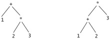
The transformation from concrete to abstract syntax takes place in two stages. First, a lexical analyzer (or lexer) converts the string of characters written by the programmer into a sequence of tokens—identifiers, keywords, constants, punctuation, etc. The lexer removes comments and deals with issues such as whitespace and capitalization conventions, and formats for numeric and string constants. Next, a parser transforms this sequence of tokens into an abstract syntax tree. During parsing, various conventions such as operator precedence and associativity reduce the need to clutter surface programs with parentheses to explicitly indicate the structure of compound expressions. For example, * binds more tightly than +, so the parser interprets the unparenthesized expression 1+2*3 as the abstract syntax tree to the left below rather than the one to the right:

The focus of attention in this book is on abstract, not concrete, syntax. Grammars like the one for lambda-terms above should be understood as describing legal tree structures, not strings of tokens or characters. Of course, when we write terms in examples, definitions, theorems, and proofs, we will need to express them in a concrete, linear notation, but we always have their underlying abstract syntax trees in mind.

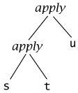
To save writing too many parentheses, we adopt two conventions when writing lambda-terms in linear form. First, application associates to the left—that is, s t u stands for the same tree as (s t) u:

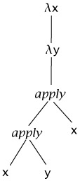
Second, the bodies of abstractions are taken to extend as far to the right as possible, so that, for example, λx. λy. x y x stands for the same tree as λx. (λy. ((x y) x)):

Variables and Metavariables

Another subtlety in the syntax definition above concerns the use of metavariables. We will continue to use the metavariable t (as well as s, and u, with or without subscripts) to stand for an arbitrary term.^[4] Similarly, x (as well as y and z) stands for an arbitrary variable. Note, here, that x is a metavariable ranging over variables! To make matters worse, the set of short names is limited, and we will also want to use x, y, etc. as object-language variables. In such cases, however, the context will always make it clear which is which. For example, in a sentence like "The term λx. λy. x y has the form λz.s, where z = x and s = λy. x y," the names z and s are metavariables, whereas x and y are object-language variables.

Scope

A final point we must address about the syntax of the lambda-calculus is the scopes of variables.

An occurrence of the variable x is said to be bound when it occurs in the body t of an abstraction λx.t. (More precisely, it is bound by this abstraction. Equivalently, we can say that λx is a binder whose scope is t.) An occurrence of x is free if it appears in a position where it is not bound by an enclosing abstraction on x. For example, the occurrences of x in x y and λy. x y are free, while the ones in λx.x and λz. λx. λy. x (y z) are bound. In (λx.x) x, the first occurrence of x is bound and the second is free.

A term with no free variables is said to be closed; closed terms are also called combinators. The simplest combinator, called the identity function,

   id = λx.x;

does nothing but return its argument.

Operational Semantics

In its pure form, the lambda-calculus has no built-in constants or primitive operators—no numbers, arithmetic operations, conditionals, records, loops, sequencing, I/O, etc. The sole means by which terms "compute" is the application of functions to arguments (which themselves are functions). Each step in the computation consists of rewriting an application whose left-hand component is an abstraction, by substituting the right-hand component for the bound variable in the abstraction's body. Graphically, we write

   (λx. t₁₂) t₂ → [x ↦ t₂]t₁₂,

where [x ↦ t₂]t₁₂ means "the term obtained by replacing all free occurrences of x in t₁₂ by t₂." For example, the term (λx.x) y evaluates to y and the term (λx. x (λx.x)) (u r) evaluates to u r (λx.x). Following Church, a term of the form (λx. t₁₂) t₂ is called a redex ("reducible expression"), and the operation of rewriting a redex according to the above rule is called beta-reduction.

Several different evaluation strategies for the lambda-calculus have been studied over the years by programming language designers and theorists. Each strategy defines which redex or redexes in a term can fire on the next step of evaluation.^[5]

Under full beta-reduction, any redex may be reduced at any time. At each step we pick some redex, anywhere inside the term we are evaluating, and reduce it. For example, consider the term
```
   (λx.x) ((λx.x) (λz. (λx.x) z)), 
```
which we can write more readably as id (id (λz. id z)). This term contains three redexes:
```
    id (id (λz. id z))    id ((id (λz. id z)))    id (id (λz. id z)) 
```
Under full beta-reduction, we might choose, for example, to begin with the innermost redex, then do the one in the middle, then the outermost:
```
        id (id (λz. id z))     →  id (id (λz.z))     →  id (λz.z)     →  λz.z     ↛ 
```
Under the normal order strategy, the leftmost, outermost redex is always reduced first. Under this strategy, the term above would be reduced as follows:
```
        id (id (λz. id z))     →  id (z. id z)     →  λz. id z     →  λz.z     ↛ 
```
Under this strategy (and the ones below), the evaluation relation is actually a partial function: each term t evaluates in one step to at most one term t′.
The call by name strategy is yet more restrictive, allowing no reductions inside abstractions. Starting from the same term, we would perform the first two reductions as under normal-order, but then stop before the last and regard λz. id z as a normal form:
```
        id (id (λz. id z))     →  id (λz. id z)     →  λz. id z     ↛ 
```
Variants of call by name have been used in some well-known programming languages, notably Algol-60 (Naur et al., 1963) and Haskell (Hudak et al., 1992). Haskell actually uses an optimized version known as call by need (Wadsworth, 1971; Ariola et al., 1995) that, instead of re-evaluating an argument each time it is used, overwrites all occurrences of the argument with its value the first time it is evaluated, avoiding the need for subsequent re-evaluation. This strategy demands that we maintain some sharing in the run-time representation of terms—in effect, it is a reduction relation on abstract syntax graphs, rather than syntax trees.
Most languages use a call by value strategy, in which only outermost redexes are reduced and where a redex is reduced only when its right-hand side has already been reduced to a value—a term that is finished computing and cannot be reduced any further.^[6] Under this strategy, our example term reduces as follows:
```
        id (id (λz. id z))     →  id (λz. id z)     →  λz. id z     ↛ 
```
The call-by-value strategy is strict, in the sense that the arguments to functions are always evaluated, whether or not they are used by the body of the function. In contrast, non-strict (or lazy) strategies such as call-by-name and call-by-need evaluate only the arguments that are actually used.

The choice of evaluation strategy actually makes little difference when discussing type systems. The issues that motivate various typing features, and the techniques used to address them, are much the same for all the strategies. In this book, we use call by value, both because it is found in most well-known languages and because it is the easiest to enrich with features such as exceptions (Chapter 14) and references (Chapter 13).

^[2]The phrase lambda-term is used to refer to arbitrary terms in the lambda-calculus. Lambda-terms beginning with a λ are often called lambda-abstractions.

^[3]Definitions of full-blown languages sometimes use even more levels. For example, following Landin, it is often useful to define the behaviors of some languages constructs as derived forms, by translating them into combinations of other, more basic, features. The restricted sublanguage containing just these core features is then called the internal language (or IL), while the full language including all derived forms is called the external language (EL). The transformation from EL to IL is (at least conceptually) performed in a separate pass, following parsing. Derived forms are discussed in Section 11.3.

^[4]Naturally, in this chapter, t ranges over lambda-terms, not arithmetic expressions. Throughout the book, t will always range over the terms of calculus under discussion at the moment. A footnote on the first page of each chapter specifies which system this is.

^[5]Some people use the terms "reduction" and "evaluation" synonymously. Others use "evaluation" only for strategies that involve some notion of "value" and "reduction" otherwise.

^[6]In the present bare-bones calculus, the only values are lambda-abstractions. Richer calculi will include other values: numeric and boolean constants, strings, tuples of values, records of values, lists of values, etc.

< Free Open Study >