3.5 Evaluation
|
| < Free Open Study > |
|
3.5 Evaluation
Leaving numbers aside for the moment, let us begin with the operational semantics of just boolean expressions. Figure 3-1 summarizes the definition. We now examine its parts in detail.
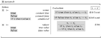
Figure 3-1: Booleans (B)
The left-hand column of Figure 3-1 is a grammar defining two sets of expressions. The first is just a repetition (for convenience) of the syntax of terms. The second defines a subset of terms, called values, that are possible final results of evaluation. Here, the values are just the constants true and false. The metavariable v is used throughout the book to stand for values.
The right-hand column defines an evaluation relation[5] on terms, written t → t′ and pronounced "t evaluates to t′ in one step." The intuition is that, if t is the state of the abstract machine at a given moment, then the machine can make a step of computation and change its state to t′. This relation is defined by three inference rules (or, if you prefer, two axioms and a rule, since the first two have no premises).
The first rule, E-IFTRUE, says that, if the term being evaluated is a conditional whose guard is literally the constant true, then the machine can throw away the conditional expression and leave the then part, t2, as the new state of the machine (i.e., the next term to be evaluated). Similarly, E-IFFALSE says that a conditional whose guard is literally false evaluates in one step to its else branch, t3. The E- in the names of these rules is a reminder that they are part of the evaluation relation; rules for other relations will have diMerent prefixes.
The third evaluation rule, E-IF, is more interesting. It says that, if the guard t1 evaluates to t′1, then the whole conditional if t1 then t2 else t3 evaluates to if t′1 then t2 else t3. In terms of abstract machines, a machine in state if t1 then t2 else t3 can take a step to state if t′1 then t2 else t3 if another machine whose state is just t1 can take a step to state t′1.
What these rules do not say is just as important as what they do say. The constants true and false do not evaluate to anything, since they do not appear as the left-hand sides of any of the rules. Moreover, there is no rule allowing the evaluation of a then-or else-subexpression of an if before evaluating the if itself: for example, the term
if true then (if false then false else false) else true
does not evaluate to if true then false else true. Our only choice is to evaluate the outer conditional first, using E-IF. This interplay between the rules determines a particular evaluation strategy for conditionals, corresponding to the familiar order of evaluation in common programming languages: to evaluate a conditional, we must first evaluate its guard; if the guard is itself a conditional, we must first evaluate its guard; and so on. The E-IFTRUE and E-IFFALSE rules tell us what to do when we reach the end of this process and find ourselves with a conditional whose guard is already fully evaluated. In a sense, E-IFTRUE and E-IFFALSE do the real work of evaluation, while E-IF helps determine where the work is to be done. The different character of the rules is sometimes emphasized by referring to E-IFTRUE and E-IFFALSE as computation rules and E-IF as a congruence rule.
To be a bit more precise about these intuitions, we can define the evaluation relation formally as follows.
3.5.1 Definition
An instance of an inference rule is obtained by consistently replacing each metavariable by the same term in the rule's conclusion and all its premises (if any).
For example,
if true then true else (if false then false else false) → true is an instance of E-IFTRUE, where both occurrences of t2 have been replaced by true and t3 has been replaced by if false then false else false.
3.5.2 Definition
A rule is satisfied by a relation if, for each instance of the rule, either the conclusion is in the relation or one of the premises is not.
3.5.3 Definition
The one-step evaluation relation → is the smallest binary relation on terms satisfying the three rules in Figure 3-1. When the pair (t, t′) is in the evaluation relation, we say that "the evaluation statement (or judgment) t → t′ is derivable.
The force of the word "smallest" here is that a statement t → t′ is derivable iff it is justified by the rules: either it is an instance of one of the axioms E-IFTRUE and E-IFFALSE, or else it is the conclusion of an instance of rule E-IF whose premise is derivable. The derivability of a given statement can be justified by exhibiting a derivation tree whose leaves are labeled with instances of E-IFTRUE or E-IFFALSE and whose internal nodes are labeled with instances of E-IF. For example, if we abbreviate
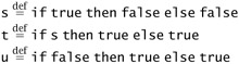
to avoid running off the edge of the page, then the derivability of the statement
if t then false else false → if u then false else false is witnessed by the following derivation tree:
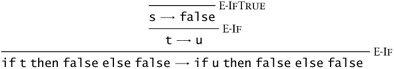
Calling this structure a tree may seem a bit strange, since it doesn't contain any branches. Indeed, the derivation trees witnessing evaluation statements will always have this slender form: since no evaluation rule has more than one premise, there is no way to construct a branching derivation tree. The terminology will make more sense when we consider derivations for other inductively defined relations, such as typing, where some of the rules do have multiple premises.
The fact that an evaluation statement t → t′ is derivable iff there is a derivation tree with t → t′ as the label at its root is often useful when reasoning about properties of the evaluation relation. In particular, it leads directly to a proof technique called induction on derivations. The proof of the following theorem illustrates this technique.
3.5.4 Theorem [Determinacy of One-Step Evaluation]
If t →t′ and t → t″, then t′ = t″.
Proof: By induction on a derivation of t → t′. At each step of the induction, we assume the desired result for all smaller derivations, and proceed by a case analysis of the evaluation rule used at the root of the derivation. (Notice that the induction here is not on the length of an evaluation sequence: we are looking just at a single step of evaluation. We could just as well say that we are performing induction on the structure of t, since the structure of an "evaluation derivation" directly follows the structure of the term being reduced. Alternatively, we could just as well perform the induction on the derivation of t → t″ instead.)
If the last rule used in the derivation of t → t′ is E-IFTRUE, then we know that t has the form if t1 then t2 else t3, where t1 = true. But now it is obvious that the last rule in the derivation of t → t″ cannot be E-IFFALSE, since we cannot have both t1 = true and t1 = false. Moreover, the last rule in the second derivation cannot be E-IF either, since the premise of this rule demands that t1 → t′1 for some t′1, but we have already observed that true does not evaluate to anything. So the last rule in the second derivation can only be E-IFTRUE, and it immediately follows that t′ = t″.
Similarly, if the last rule used in the derivation of t → t′ is E-IFFALSE, then the last rule in the derivation of t → t″ must be the same and the result is immediate.
Finally, if the last rule used in the derivation of t → t′ is E-IF, then the form of this rule tells us that t has the form if t1 then t2 else t3, where t1 → t′1 for some t′1. By the same reasoning as above, the last rule in the derivation of t → t″ can only be E-IF, which tells us that t has the form if t1 then t2 else t3 (which we already know) and that t1 → t″1 for some t″1. But now the induction hypothesis applies (since the derivations of t1 → t′1 and t1 → t″1 are subderivations of the original derivations of t → t′ and t → t″), yielding t′1 = t″1. This tells us that t′ = if t′1 then t2 else t3 = if t″1 then t2 else t3 = t″, as required.
3.5.5 Exercise [⋆]
Spell out the induction principle used in the preceding proof, in the style of Theorem 3.3.4.
Our one-step evaluation relation shows how an abstract machine moves from one state to the next while evaluating a given term. But as programmers we are just as interested in the final results of evaluation—i.e., in states from which the machine cannot take a step.
3.5.6 Definition
A term t is in normal form if no evaluation rule applies to it—i.e., if there is no t′ such that t → t′. (We sometimes say "t is a normal form" as shorthand for "t is a term in normal form.")
We have already observed that true and false are normal forms in the present system (since all the evaluation rules have left-hand sides whose outermost constructor is an if, there is obviously no way to instantiate any of the rules so that its left-hand side becomes true or false). We can rephrase this observation in more general terms as a fact about values:
3.5.7 Theorem
Every value is in normal form.
When we enrich the system with arithmetic expressions (and, in later chapters, other constructs), we will always arrange that Theorem 3.5.7 remains valid: being in normal form is part of what it is to be a value (i.e., a fully evaluated result), and any language definition in which this is not the case is simply broken.
In the present system, the converse of Theorem 3.5.7 is also true: every normal form is a value. This will not be the case in general; in fact, normal forms that are not values play a critical role in our analysis of run-time errors, as we shall see when we get to arithmetic expressions later in this section.
3.5.8 Theorem
If t is in normal form, then t is a value.
Proof: Suppose that t is not a value. It is easy to show, by structural induction on t, that it is not a normal form.
Since t is not a value, it must have the form if t1 then t2 else t3 for some t1, t2, and t3. Consider the possible forms of t1.
If t1 = true, then clearly t is not a normal form, since it matches the left-hand side of E-IFTRUE. Similarly if t1 = false.
If t1 is neither true nor false, then it is not a value. The induction hypothesis then applies, telling us that t1 is not a normal form—that is, that there is some t′1 such that t1 → t′1. But this means we can use E-IF to derive t → if t′1 then t2 else t3, so t is not a normal form either.
It is sometimes convenient to be able to view many steps of evaluation as one big state transition. We do this by defining a multi-step evaluation relation that relates a term to all of the terms that can be derived from it by zero or more single steps of evaluation.
3.5.9 Definition
The multi-step evaluation relation →* is the reflexive, transitive closure of one-step evaluation. That is, it is the smallest relation such that (1) if t → t′ then t →* t′, (2) t →* t for all t, and (3) if t →* t′ and t′ →* t″, then t →* t″.
3.5.10 Exercise [⋆]
Rephrase Definition 3.5.9 as a set of inference rules.
Having an explicit notation for multi-step evaluation makes it easy to state facts like the following:
3.5.11 Theorem [Uniqueness of Normal Forms]
If t →* u and t →* u′, where u and u′ are both normal forms, then u = u′.
Proof: Corollary of the determinacy of single-step evaluation (3.5.4).
The last property of evaluation that we consider before turning our attention to arithmetic expressions is the fact that every term can be evaluated to a value. Clearly, this is another property that need not hold in richer languages with features like recursive function definitions. Even in situations where it does hold, its proof is generally much more subtle than the one we are about to see. In Chapter 12 we will return to this point, showing how a type system can be used as the backbone of a termination proof for certain languages.
Most termination proofs in computer science have the same basic form:[6] First, we choose some well-founded set S and give a function f mapping "machine states" (here, terms) into S. Next, we show that, whenever a machine state t can take a step to another state t′, we have f(t′) < f(t). We now observe that an infinite sequence of evaluation steps beginning from t can be mapped, via f, into an infinite decreasing chain of elements of S. Since S is well founded, there can be no such infinite decreasing chain, and hence no infinite evaluation sequence. The function f is often called a termination measure for the evaluation relation.
3.5.12 Theorem [Termination of Evaluation]
For every term t there is some normal form t′ such that t →* t′.
Proof: Just observe that each evaluation step reduces the size of the term and that size is a termination measure because the usual order on the natural numbers is well founded.
3.5.13 Exercise [Recommended, ⋆⋆]
-
Suppose we add a new rule

to the ones in Figure 3-1. Which of the above theorems (3.5.4, 3.5.7, 3.5.8, 3.5.11, and 3.5.12) remain valid?
-
Suppose instead that we add this rule:

Now which of the above theorems remain valid? Do any of the proofs need to change?
Our next job is to extend the definition of evaluation to arithmetic expressions. Figure 3-2 summarizes the new parts of the definition. (The notation in the upper-right corner of 3-2 reminds us to regard this figure as an extension of 3-1, not a free-standing language in its own right.)
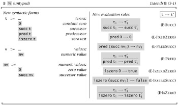
Figure 3-2: Arithmetic Expressions (NB)
Again, the definition of terms is just a repetition of the syntax we saw in §3.1. The definition of values is a little more interesting, since it requires introducing a new syntactic category of numeric values. The intuition is that the final result of evaluating an arithmetic expression can be a number, where a number is either 0 or the successor of a number (but not the successor of an arbitrary value: we will want to say that succ(true) is an error, not a value).
The evaluation rules in the right-hand column of Figure 3-2 follow the same pattern as we saw in Figure 3-1. There are four computation rules (E-PREDZERO, E-PREDSUCC, E-ISZEROZERO, and E-ISZEROSUCC) showing how the operators pred and iszero behave when applied to numbers, and three congruence rules (E-SUCC, E-PRED, and E-ISZERO) that direct evaluation into the "first" subterm of a compound term.
Strictly speaking, we should now repeat Definition 3.5.3 ("the one-step evaluation relation on arithmetic expressions is the smallest relation satisfying all instances of the rules in Figures 3-1 and 3-2..."). To avoid wasting space on this kind of boilerplate, it is common practice to take the inference rules as constituting the definition of the relation all by themselves, leaving "the smallest relation containing all instances..." as understood.
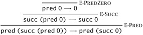
The syntactic category of numeric values (nv) plays an important role in these rules. In E-PREDSUCC, for example, the fact that the left-hand side is pred (succ nv1) (rather than pred (succ t1), for example) means that this rule cannot be used to evaluate pred (succ (pred 0)) to pred 0, since this would require instantiating the metavariable nv1 with pred 0, which is not a numeric value. Instead, the unique next step in the evaluation of the term pred (succ (pred 0)) has the following derivation tree:
3.5.14 Exercise [⋆⋆]
Show that Theorem 3.5.4 is also valid for the evaluation relation on arithmetic expressions: if t → t′ and t → t″, then t′ = t″.
Formalizing the operational semantics of a language forces us to specify the behavior of all terms, including, in the case at hand, terms like pred 0 and succ false. Under the rules in Figure 3-2, the predecessor of 0 is defined to be 0. The successor of false, on the other hand, is not defined to evaluate to anything (i.e., it is a normal form). We call such terms stuck.
3.5.15 Definition
A closed term is stuck if it is in normal form but not a value.
"Stuckness" gives us a simple notion of run-time error for our simple machine. Intuitively, it characterizes the situations where the operational semantics does not know what to do because the program has reached a "meaningless state." In a more concrete implementation of the language, these states might correspond to machine failures of various kinds: segmentation faults, execution of illegal instructions, etc. Here, we collapse all these kinds of bad behavior into the single concept of "stuck state."
3.5.16 Exercise [Recommended, ⋆⋆⋆]
A different way of formalizing meaningless states of the abstract machine is to introduce a new term called wrong and augment the operational semantics with rules that explicitly generate wrong in all the situations where the present semantics gets stuck. To do this in detail, we introduce two new syntactic categories
|
badnat ::= wrong true false badbool ::= wrong nv | non-numeric normal forms: run-time error constant true constant false non-boolean normal forms: run-time error numeric value |
and we augment the evaluation relation with the following rules:
![]()
![]()
![]()
![]()
Show that these two treatments of run-time errors agree by (1) finding a precise way of stating the intuition that "the two treatments agree," and (2) proving it. As is often the case when proving things about programming languages, the tricky part here is formulating a precise statement to be proved—the proof itself should be straightforward.
3.5.17 Exercise [Recommended, ⋆⋆⋆]
Two styles of operational semantics are in common use. The one used in this book is called the small-step style, because the definition of the evaluation relation shows how individual steps of computation are used to rewrite a term, bit by bit, until it eventually becomes a value. On top of this, we define a multi-step evaluation relation that allows us to talk about terms evaluating (in many steps) to values. An alternative style, called big-step semantics (or sometimes natural semantics), directly formulates the notion of "this term evaluates to that final value," written t ⇓ v. The big-step evaluation rules for our language of boolean and arithmetic expressions look like this:
![]()
![]()
![]()
![]()
![]()
![]()
![]()
![]()
Show that the small-step and big-step semantics for this language coincide, i.e. t →* v iff t ⇓ v.
3.5.18 Exercise [⋆⋆ ↛]
Suppose we want to change the evaluation strategy of our language so that the then and else branches of an if expression are evaluated (in that order) before the guard is evaluated. Show how the evaluation rules need to change to achieve this effect.
[5]Some experts prefer to use the term reduction for this relation, reserving evaluation for the "big-step" variant described in Exercise 3.5.17, which maps terms directly to their final values.
[6]In Chapter 12 we will see a termination proof with a somewhat more complex structure.
|
| < Free Open Study > |
|
EAN: 2147483647
Pages: 262