A.9 Proposition

< Free Open Study >

If t →* v then t ⇓ v.

Proof: By induction on the number of steps of small-step evaluation in the given derivation of t →* v.

If t →* v in 0 steps, then t = v and the result follows by B-VALUE. Otherwise, we proceed by case analysis on the form of t.

Case:

t = if t₁ then t₂ else t₃

By Lemma A.8, either (1) t₁ →* true and t₂ →* v or (2) t₁ →* false and t₃ →* v. The arguments in both cases are similar, so suppose we have case (1). Lemma A.8 also tells us that the evaluation sequences for t₁ →* true and t₂ →* v are shorter than the given one for t, so the induction hypothesis applies, giving us t₁ ⇓ true and t₂ ⇓ v. From these, we can use rule B-IFTRUE to derive t ⇓ v.

The cases for the other term constructors are similar.

4.2.1 Solution

Each time eval calls itself, it adds a try handler to the call stack. Since there is one recursive call for each step of evaluation, the stack will eventually overflow. In essence, wrapping the recursive call to eval in a try means that it is not a tail call, although it looks like one. A better (but less readable) version of eval is:

   let rec eval t =     let t'opt = try $(eval1 t) with NoRuleApplies → None in     match t'opt with       $(t') → eval t'     | None → t

5.2.1 Solution

   or = λb. λc. b tru c;   not = λb. b fls tru;

5.2.2 Solution

   scc2 = λn. λs. λz. n s (s z);

5.2.3 Solution

   times2 = λm. λn. λs. λz. m (n s) z;

Or, more compactly:

   times3 = λm. λn. λs. m (n s);

5.2.4 Solution

Again, there is more than one way to do it:

   power1 = λm. λn. m (times n) c₁;   power2 = λm. λn. m n;

5.2.5 Solution

   subtract1 = λm. λn. n prd m;

5.2.6 Solution

Evaluating prd c_n takes O(n) steps, since prd uses n to construct a sequence of n pairs of numbers and then selects the first component of the last pair of the sequence.

5.2.7 Solution

Here's a simple one:

   equal = λm. λn.             and (iszro (m prd n))                 (iszro (n prd m));

5.2.8 Solution

This is the solution I had in mind:

   nil = λc. λn. n;   cons = λh. λt. λc. λn. c h (t c n);   head = λl. l (λh.λt.h) fls;   tail = λl.            fst (l (λx. λp. pair (snd p) (cons x (snd p)))                   (pair nil nil));   isnil = λl. l (λh.λt.fls) tru;

Here is a rather different approach:

   nil = pair tru tru;   cons = λh. λt. pair fls (pair h t);   head = λz. fst (snd z);   tail = λz. snd (snd z);   isnil = fst;

5.2.9 Solution

We used if rather than test to prevent both branches of the conditional always being evaluated, which would make factorial diverge. To prevent this divergence when using test, we need to protect both branches by wrapping them in dummy lambda-abstractions. Since abstractions are values, our call-by-value evaluation strategy does not look underneath them, but instead passes them verbatim to test, which chooses one and passes it back. We then apply the whole test expression to a dummy argument, say c₀, to force evaluation of the chosen branch.

   ff = λf. λn.          test            (iszro n) (λx. c₁) (λx. (times n (f (prd n)))) c₀;   factorial = fix ff;   equal c₆ (factorial c₃); ▸ (λx. λy. x)

5.2.10 Solution

Here's a recursive function that does the job:

   cn = λf. λm. if iszero m then c₀ else scc (f (pred m));   churchnat = fix cn;

A quick test that it works:

   equal (churchnat 4) c₄; ▸ (λx. λy. x)

5.2.11 Solution

   ff = λf. λl.          test (isnil l)             (λx. c₀) (λx. (plus (head l) (f (tail l)))) c₀;   sumlist = fix ff;   l = cons c₂ (cons c₃ (cons c₄ nil));   equal (sumlist l) c₉; ▸ (λx. λy. x)

A list-summing function can also, of course, be written without using fix:

   sumlist' = λl. l plus c₀;   equal (sumlist l) c₉; ▸ (λx. λy. x)

5.3.3 Solution

By induction on the size of t. Assuming the desired property for terms smaller than t, we must prove it for t itself; if we succeed, we may conclude that the property holds for all t. There are three cases to consider:

Case:

t = x

Immediate: |FV(t)| = |{x}| = 1 = size(t).

Case:

t = λx.t₁

By the induction hypothesis, |FV(t₁)| ≤ size(t₁). We now calculate as follows: |FV(t)| = |FV(t₁) \ {x}| ≤ |FV(t₁)| ≤ size(t₁) < size(t).

Case:

t = t₁ t₂

By the induction hypothesis, |FV(t₁)| ≤ size(t₁) and |FV(t₂)| ≤ size(t₂). We now calculate as follows: |FV(t)| = |FV(t₁) È FV(t₂)| ≤ |FV(t₁)| + |FV(t₂)| ≤ size(t₁) + size(t₂) < size(t).

5.3.6 Solution

For full (non-deterministic) beta-reduction, the rules are:

(Note that the syntactic category of values is not used.)

For the normal-order strategy, one way of writing the rules is

where the syntactic categories of normal forms, non-abstraction normal forms, and non-abstractions are defined as follows:

 nf ::=         λx.nf        nanf

normal forms:

 nanf ::=         x         nanf nf

non-abstraction normal forms:

 na ::=        x        t₁t₂

non-abstractions:

(This definition is a bit awkward compared to the others. Normal-order reduction is usually defined by just saying "it's like full beta-reduction, except that the left-most, outermost redex is always chosen first.")

The lazy strategy defines values as arbitrary abstractions-the same as call by value. The evaluation rules are:

5.3.8 Solution

6.1.1 Solution

   c₀ = λ. λ. 0;   c₂ = λ. λ. 1 (1 0);   plus = λ. λ. λ. λ. 3 1 (2 0 1);   fix = λ. (λ. 1 (λ. (1 1) 0)) (λ. 1 (λ. (1 1) 0));   foo = (λ. (λ. 0)) (λ. 0);

6.1.5 Solution

The two functions can be defined as follows:

removenames_Г(x)	=	the index of the rightmost x in Г
removenames_Г(λx.t₁)	=	λ. removenames_Г,x(t₁)
removenames_Г(t₁ t₂)	=	removenames_Г,x(t₁) removenames_Г,x(t₂)
restorenames_Г(k)	=	the kth name in Г
restorenames_Г(λ.t₁)	=	λx. restorenames_Г,x(t₁) where x is the first name not in dom(Г)
restorenames_Г(t₁ t₂)	=	restorenames_Г,x(t₁) restorenames_Г,x(t₂)

The required properties of removenames and restorenames are proved by straightforward structural induction on terms.

6.2.2 Solution

λ. λ. 1 (0 4)
λ. 0 3 (λ. 0 1 4)

6.2.5 Solution

[0 ↦ 1] (0 (λ.λ.2))

i.e.,

1 (λ. λ. 3)

a (λx. λy. a)

[0 ↦ 1 (λ.2)] (0 (λ.1))

i.e.,

(1 (λ.2)) (λ.(2 (λ.3)))

(a (λz.a)) (λx.(a (λz.a)))

[0 ↦ 1] (λ. 0 2)

i.e.,

λ. 0 2

λb. b a

[0 ↦ 1] (λ. 1 0)

i.e.,

λ. 2 0

λa′. a a′

6.2.8 Solution

If Г is a naming context, write Г(x) for the index of x in Г, counting from the right. Now, the property that we want is that

removenames_Г([x ↦ s]t) = [Г(x) ↦ removenames_Г(s)](removenames_Г(t)).

The proof proceeds by induction on t, using Definitions 5.3.5 and 6.2.4, some simple calculations, and some easy lemmas about removenames and the other basic operations on terms. Convention 5.3.4 plays a crucial role in the abstraction case.

6.3.1 Solution

The only way an index could become negative would be if the variable numbered 0 actually occurred anywhere in the term we shift. But this cannot happen, since we've just performed a substitution for variable 0 (and since the term that we substituted for variable 0 was already shifted up, so it obviously cannot contain any instances of variable number 0).

6.3.2 Solution

The proof of equivalence of the presentations using indices and levels can be found in Lescanne and Rouyer-Degli (1995). De Bruijn levels are also discussed by de Bruijn (1972) and Filinski (1999, Section 5.2).

8.3.5 Solution

No: removing this rule breaks the progress property. If we really object to defining the predecessor of 0, we need to handle it in another way-e.g., by raising an exception (Chapter 14) if a program attempts it, or refining the type of pred to make clear that it can legally be applied only to strictly positive numbers, perhaps using intersection types (§15.7) or dependent types (§30.5).

8.3.6 Solution

Here's a counterexample: the term (if false then true else 0) is ill-typed, but evaluates to the well-typed term 0.

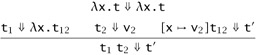
8.3.7 Solution

The type preservation property for the big-step semantics is similar to the one we gave for the small-step semantics: if a well-typed term evaluates to some final value, then this value has the same type as the original term. The proof is similar to the one we gave. The progress property, on the other hand, now makes a much stronger claim: it says that every well-typed term can be evaluated to some final value-that is, that evaluation always terminates on well-typed terms. For arithmetic expressions, this happens to be the case, but for more interesting languages (languages involving general recursion, for example-cf. §11.11) it will often not be true. For such languages, we simply have no progress property: in effect, there is no way to tell the difference between reaching an error state and failing to terminate. This is one reason that language theorists generally prefer the small-step style.

A different alternative is to give a big-step semantics with explicit wrong transitions, in the style of Exercise 8.3.8. This style is used, for example, by Abadi and Cardelli for the operational semantics of their object calculus (Abadi and Cardelli, 1996, p. 87).

8.3.8 Solution

In the augmented semantics there are no stuck states at all-every non-value term either evaluates to another term in the ordinary way or else goes explicitly to wrong (this must be proved, of course)-so the progress property is trivial. The subject-reduction theorem, on the other hand, now tells us a little more. Since wrong has no type, saying that a well-typed term can evaluate only to another well-typed term tells us, in particular, that a well-typed term cannot take a step to wrong. In effect, the proof of the old progress theorem becomes part of the new proof of preservation.

9.2.1 Solution

Because the set of type expressions is empty (there is no base case in the syntax of types).

9.2.3 Solution

One such context is

   Г = f:Bool→Bool→Bool, x:Bool, y:Bool.

In general, any context of the form

   Г = f:S→T→Bool, x:S, y:T

where S and T are arbitrary types, will do the job. This sort of reasoning is central to the type reconstruction algorithm developed in Chapter 22.

9.4.1 Solution

T-TRUE and T-FALSE are introduction rules. T-IF is an elimination rule. T-ZERO and T-SUCC are introduction rules. T-PRED and T-ISZERO are elimination rules. Deciding whether succ and pred are introduction or elimination forms requires a little thought, since they can be viewed as both creating and using numbers. The key observation is that, when pred and succ meet, they make a redex. Similarly for iszero.

9.3.2 Solution

Suppose, for a contradiction, that the term x x does have a type T. Then, by the inversion lemma, the left-hand subterm (x) must have a type T₁→T₂ and the right-hand subterm (also x) must have type T₁. Using the variable case of the inversion lemma, we find that x:T₁→T₂ and x:T₁ must both come from assumptions in Г. Since there can only be one binding for x in Г, this means that T₁→T₂ = T₁. But this means that size(T₁) is strictly greater than size(T₁→T₂), an impossibility, and we have our contradiction.

Notice that if types were allowed to be infinitely large, then we could construct a solution to the equation T₁→T₂ = T₁. We will return to this point in detail in Chapter 20.

9.3.3 Solution

Suppose that Г ⊢ t : S and Г ⊢ t : T. We show, by induction on a derivation of Г ⊢ t : T, that S = T.

Case T-VAR:

t = x

with x:T Î Г

By case (1) of the inversion lemma (9.3.1), the final rule in any derivation of Г ⊢ t : S must also be T-VAR, and S = T.

Case T-ABS:

t = λy:T₂.t₁

T = T₂→T₁

Г, y:T₂ ⊢ t₁ : T₁

By case (2) of the inversion lemma, the final rule in any derivation of Г ⊢ t : S must also be T-ABS, and this derivation must have a subderivation with conclusion Г, y:T₂ ⊢ t₁ : S₁, with S = T₂→S₁. By the induction hypothesis (on the subderivation with conclusion (Г, y:T₂ ⊢ t₁ : T₁), we obtain S₁ = T₁, from which S = T is immediate.

Case T-APP, T-TRUE, T-FALSE, T-IF:

Similar.

9.3.9 Solution

By induction on a derivation of Г ⊢ t : T. At each step of the induction, we assume that the desired property holds for all subderivations (i.e., that if Г ⊢ s : S and s → s′, then Г ⊢ s′ : S whenever Г ⊢ s : S is proved by a subderivation of the present one) and proceed by case analysis on the last rule used in the derivation.

Case T-VAR:

t = x

x:T Î Г

Can't happen (there are no evaluation rules with a variable as the left-hand side).

Case T-ABS:

t = λx:T₁ . t₂

Can't happen.

Case T-APP:

t = t₁ t₂

T = T₁₂

Г ⊢ t₁ : T₁₁→T₁₂

Г ⊢ t₂ :T₁₁

Looking at the evaluation rules in Figure 9-1 with applications on the lefthand side, we find that there are three rules by which t → t′ can be derived: E-APP1, E-APP2, and E-APPABS. We consider each case separately.

Subcase E-APP1:
From the assumptions of the T-APP case, we have a subderivation of the original typing derivation whose conclusion is Г ⊢ t₁ : T₁₁→T₁₂. We can apply the induction hypothesis to this subderivation, obtaining . Combining this with the fact (also from the assumptions of the T-APP case) that Г ⊢ t₂ : T₁₁, we can apply rule T-APP to conclude that Г ⊢ t′ : T.
Subcase E-APP2:

t₁ = v₁ (i.e., t₁ is a value)
Similar.
Subcase E-APPABS:

t₁ = λx:T₁₁. t₁₂

t₂ = v₂

t′ = [x ↦ v₂]t₁₂
Using the inversion lemma, we can deconstruct the typing derivation for λx:T₁₁. t₁₂, yielding Г, x:T₁₁ ⊢ t₁₂ : T₁₂. From this and the substitution lemma (9.3.8), we obtain Г ⊢ t′ : T₁₂.

The cases for boolean constants and conditional expressions are the same as in 8.3.3.

9.3.10 Solution

The term (λx:Bool. λy:Bool. y) (true true) is ill typed, but reduces to (λy:Bool.y), which is well typed.

11.2.1 Solution

t₁	=	(λx:Unit.x) unit
t_i+1	=	(λf:Unit→Unit. f(f(unit))) (λx:Unit.t_i)

11.3.2 Solution

The proof that these rules are derived from the abbreviation goes exactly like Theorem 11.3.1.

11.4.1 Solution

The first part is easy: if we desugar ascription using the rule t as T = (λx:T. x) t,x then it is straightforward to check that both the typing and the evaluation rules for ascription can be derived directly from the rules for abstraction and application.

If we change the evaluation rule for ascription to an eager version, then we need a more refined desugaring that delays evaluation of t until after the ascription has been thrown away. For example, we can use this one:

Of course, the choice of Unit here is inessential: any type would do.

The subtlety here is that this desugaring, though intuitively correct, does not give us exactly the properties of Theorem 11.3.1. The reason is that a desugared ascription takes two steps of evaluation to disappear, while the high-level rule E-ASCRIBE works in a single step. However, this should not surprise us: we can think of this desugaring as a simple form of compilation, and observe that the compiled forms of nearly every high-level construct require multiple steps of evaluation in the target language for each atomic reduction in the source language. What we should do, then, is weaken the requirements of 11.3.1 to demand only that each high-level evaluation step should be matched by some sequence of low-level steps:

if t →_E t′, then e(t) →*_Ie(t′).

A final subtlety is that the other direction-i.e., the fact that reductions of a desugared term can always be "mapped back" to reductions of the original term-requires a little care to state precisely, since the elimination of a desugared ascription takes two steps, and after the first step the low-level term does not correspond to the desugaring of either the original term with a high-level ascription or the term in which it has been eliminated. What is true, though, is that the first reduction of a desugared term can always be "completed" by taking it one more step to reach the desugaring of another high-level term. Formally, if e(t) →_I s, then s →* e(t′), with t →_E t′.

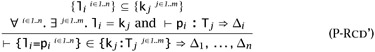
11.5.1 Solution

Here is what you need to add:

   let rec eval1 ctx t = match t with       ...     | TmLet(fi,x,v1,t2) when isval ctx v1 →         termSubstTop v1 t2     | TmLet(fi,x,t1,t2) →         let t1' = eval1 ctx t1 in         TmLet(fi, x, t1', t2)       ...   let rec typeof ctx t =     match t with       ...     | TmLet(fi,x,t1,t2) →        let tyT1 = typeof ctx t1 in        let ctx' = addbinding ctx x (VarBind(tyT1)) in        (typeof ctx' t2)

11.5.2 Solution

This definition doesn't work very well. For one thing, it changes the order of evaluation: the rules E-LETV and E-LET specify a call-by-value order, where t₁ in let x=t₁ in t₂ must be reduced to a value before we are allowed to substitute it for x and begin working on t₂. For another thing, although the validity of the typing rule T-LET is preserved by this translation-this follows directly from the substitution lemma (9.3.8)-the property of ill-typedness of terms is not preserved. For example, the ill-typed term

   let x = unit(unit) in unit

is translated to the well-typed term unit: since x does not appear in the body unit, the ill-typed subterm unit(unit) simply disappears.

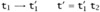
11.8.2 Solution

One proposal for adding types to record patterns is summarized in Figure A-1. The typing rule for the generalized let construct, T-LET, refers to a separate "pattern typing" relation that (viewed algorithmically) takes a pattern and a type as input and, if it succeeds, returns a context giving appropriate bindings for the variables in the pattern. T-LET adds this context to the current context Г during the typechecking of the body t₂. (We assume throughout that the sets of variables bound by different fields of a record pattern are disjoint.)

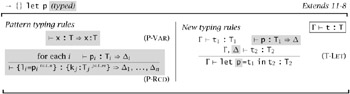
Figure A-1: Typed Record Patterns

Note that we can, if we like, refine the record pattern typing rule a little, allowing the pattern to mention fewer fields than will actually be provided by the value it will match:

If we adopt this rule, we can eliminate the record projection form as a primitive construct, since it can now be treated as syntactic sugar:

Proving preservation for the extended system is almost the same as for the simply typed lambda-calculus. The only extension that we need is a lemma connecting the pattern typing relation with the run-time matching operation. If σ is a substitution and Δ is a context with the same domain as σ, then Г ⊢ σ ⊧ Δ means that, for each x Î dom(Δ), we have Г ⊢ σ(x) : Δ(x).

LEMMA: If Г ⊢ t : T and ⊢ p : T ⇒ Δ, then match(p, t) = σ with Г ⊢ σ ⊧ Δ.

The extra notations we've introduced require a slight generalization of the standard substitution lemma (9.3.8):

LEMMA: Г, Δ ⊢ t : T and Г ⊢ σ ⊧ Δ, then Г ⊢ σ t : T.

The preservation argument for the C-LET rule now follows the same pattern as before, using these lemmas for the C-LET case.

11.9.1 Solution

Bool		Unit+Unit
true		inl unit
false		inr unit
if t₀ then t₁ else t₂		case t₀ of inl x₁ ⇒ t₁ \| inr x₂ ⇒ t₂ where x₁ and x₂ are fresh.

11.11.1 Solution

   equal =     fix       (λeq:Nat→Nat→Bool.          λm:Nat. λn:Nat.            if iszero m then iszero n            else if iszero n then false            else eq (pred m) (pred n)); ▸ equal : Nat → Nat → Bool plus = fix (λp:Nat→Nat→Nat.                 λm:Nat. λn:Nat.                   if iszero m then n else succ (p (pred m) n)); ▸ plus : Nat → Nat → Nat   times = fix (λt:Nat→Nat→Nat.                  λm:Nat. λn:Nat.                    if iszero m then 0 else plus n (t (pred m) n)); ▸ times : Nat → Nat → Nat   factorial = fix (λf:Nat→Nat.                     λm:Nat.                      if iszero m then 1 else times m (f (pred m))); ▸ factorial : Nat → Nat   factorial 5; ▸ 120 : Nat

11.11.2 Solution

   letrec plus : Nat→Nat→Nat =     λm:Nat. λn:Nat.       if iszero m then n else succ (plus (pred m) n) in   letrec times : Nat→Nat→Nat =     λm:Nat. λn:Nat.       if iszero m then 0 else plus n (times (pred m) n) in   letrec factorial : Nat→Nat =     λm:Nat.       if iszero m then 1 else times m (factorial (pred m)) in   factorial 5; ▸ 120 : Nat

11.12.1 Solution

Surprise! Actually, the progress theorem does not hold. For example, the expression head[T] nil[T] is stuck-no evaluation rule applies to it, but it is not a value. In a full-blown programming language, this situation would be handled by making head[T] nil[T] raise an exception rather than getting stuck: we consider exceptions in Chapter 14.

11.12.2 Solution

Not quite all: if we erase the annotation on nil, then we lose the Uniqueness of Types theorem. Operationally, when the typechecker sees a nil it knows it has to assign it the type List T for some T, but it does not know how to choose T without some form of guessing. Of course, more sophisticated typing algorithms such as the one used by the OCaml compiler do precisely this sort of guessing. We will return to this point in Chapter 22.

12.1.1 Solution

In the case for applications. Suppose we are trying to show that t₁ t₂ is normalizing. We know by the induction hypothesis that both t₁ and t₂ are normalizing; let v₁ and v₂ be their normal forms. By the inversion lemma for the typing relation (9.3.1), we know that v₁ has type T₁₁→T₁₂ for some T₁₁ and T₁₂. So, by the canonical forms lemma (9.3.4), v₁ must have the form λx:T₁₁.t₁₂. But reducing t₁ t₂ to (λx:T₁₁.t₁₂) v₂ does not give us a normal form, since the E-APPABS rule now applies, yielding [x ↦ v₂]t₁₂, so to finish the proof we must argue that this term is normalizable. But here we get stuck, since this term may, in general, be bigger than the original term t₁ t₂ (because the substitution can make as many copies of v₂ as there are occurrences of x in t₁₂).

12.1.7 Solution

Definition 12.1.2 is extended with two additional clauses:

R_Bool(t) iff t halts.
iff t halts, , and .

The proof of Lemma 12.1.4 is extended with one additional case:

Suppose that T = T₁ × T₂ for some T₁ and T₂. For the "only if" direction () we suppose that R_T(t) and we must show R_T(t′), where t → t′. We know that and from the definition of . But the evaluation rules E-PROJ1 and E-PROJ2 tell us that t.1 → t′.1 and t.2 → t′.2, so, by the induction hypothesis, and . From these, the definition of yields . The "if" direction is similar.

Finally, we need to add some cases (one for each new typing rule) to the proof of Lemma 12.1.5:

Case T-IF:	t = if t₁ then t₂ else t₃ Г ⊢ t₁ : Bool
	Г ⊢ t₂ : T	Г ⊢ t₃ : T
	where Г = x₁ : T₁, ..., x_n:T_n

Let σ = [x₁ ↦ v₁] ··· [x_n ↦ v_n]. By the induction hypothesis, we have R_Bool(σt₁), R_T(σt₂), and R_T(σt₃). By Lemma 12.1.3, σt₁, σt₂, and σt₃ are all normalizing; let us write v₁, v₂, and v₃ for their values. Lemma 12.1.4 gives us R_Bool(v₁), R_T(v₂), and R_T(v₃). Also, σt itself is clearly normalizing.

We now continue by induction on T.

If T = A or T = Bool, then R_T(σt) follows immediately from the fact that σt is normalizing.
If T = T₁→T₂, then we must show for an arbitrary . So suppose . Then, by the evaluation rules for if expressions, we see that either σt s →* v₂ s or else σt →* v₃ s, depending on whether v₁ is true or false. But we know that and by the definition of and the fact that both and . By Lemma 12.1.4, , as required.

Case T-TRUE:

t = true

T = Bool

Immediate.

Case T-FALSE:

t = false

T = Bool

Immediate.

Case T-PAIR:

t = {t₁, t₂}

Г ⊢ t₁ : T₁

Г ⊢ t₂ : T₂

T = T₁ × T₂

By the induction hypothesis, for i = 1,2. Let v_i be the normal form of each σt_i. Note, by Lemma 12.1.4, that .

The evaluation rules for the first and second projections tell us that {σt₁, σt₂} . i →* v_i, from which we obtain, by Lemma 12.1.4, that . The definition of yields , that is, .

Case T-PROJ1:

t = t₀ .1

Г ⊢ t₀ : T₁ × T₂

T = T₁

Immediate from the definition of .

13.1.1 Solution

13.1.2 Solution

No-calls to lookup with any index other than the one given to update will now diverge. The point is that we need to make sure we look up the value stored in a before we overwrite it with the new function. Otherwise, when we get around to doing the lookup, we will find the new function, not the original one.

13.1.3 Solution

Suppose the language provides a primitive free that takes a reference cell as argument and releases its storage so that (say) the very next allocation of a reference cell will obtain the same piece of memory. Then the program

   let r = ref 0 in   let s = r in   free r;   let t = ref true in   t := false;   succ (!s)

will evaluate to the stuck term succ false. Note that aliasing plays a crucial role here in setting up the problem, since it prevents us from detecting invalid deallocations by simply making free r illegal if the variable r appears free in the remainder of the expression.

This sort of example is easy to mimic in a language like C with manual memory management (our ref constructor corresponds to C's malloc, our free to a simplified version of C's free).

13.3.1 Solution

A simple account of garbage collection might go like this.

Model the finiteness of memory by taking the set L of locations to be finite.
Define reachability of locations in the store as follows. Write locations(t) for the set of locations mentioned in t. Say that a location l′ is reachable in one step from a location l in a store μ if l′ Î locations(μ(l)). Say that l′ is reachable from l if there is a finite sequence of locations beginning with l and ending with l′, with each reachable in one step from the previous one. Finally, define the set of locations reachable from a term t in a store μ, written reachable(t, μ) as the locations reachable in μ from locations(t).
Model the action of garbage collection as a relation t | μ → _gc t | μ′ defined by the following rule:

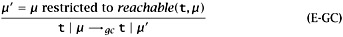
(That is, the domain of μ′ is just reachable(t, μ), and its value on every location in this domain is the same as that of μ.)
Define evaluation sequences to be sequences of ordinary evaluation steps interleaved with garbage collection 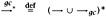. Note that we do not want to just add the rule GC to the ordinary single-step evaluation relation: it is important that we perform garbage collection only "at the outermost level," where we can see the whole term being evaluated. If we allowed garbage collection "inside" of the evaluation of the left-hand side of an application, for example, we might incorrectly re-use locations that are actually mentioned in the right-hand side of the application, since by looking at the left-hand side we would not be able to see that they were still accessible.
Justify these refinements to the definition of evaluation by showing that they do not affect final results, except for introducing the possibility of memory exhaustion:
1. If , then t | μ →* t′ | μ′, for some μ′ such that μ′ has a larger domain than μ″ and the two coincide where both are defined.
2. If t | μ →* t′ | μ′, then either
  1. , for some μ″ such that μ″ has a smaller domain than μ′ and coincides with μ′ where μ′ is defined, or else
  2. evaluation of t | μ runs out of memory-i.e., reaches a state t′″ | μ′″′″, where the next step of evaluating t′″ needs to allocate a fresh location, but none is available because reachable(t′″, μ‴) = L.

This simple treatment of garbage collection ignores several aspects of real stores, such as the fact that storing different kinds of values typically requires different amounts of memory, as well as some more advanced language features, such as finalizers (pieces of code that will be executed when the run-time system is just about to garbage collect a data structure to which they are attached) and weak pointers (pointers that are not counted as "real references" to a data structure, so that the structure may be garbage collected even though weak pointers to it still exist). A more sophisticated treatment of garbage collection in operational semantics can be found in Morrisett et al. (1995).

13.4.1 Solution

   let r₁ = ref (λx:Nat.0) in   let r₂ = ref (λx:Nat.(!r₁)x) in   (r₁ := (λx:Nat.(!r₂)x);   r₂);

13.5.2 Solution

Let μ be a store with a single location l

   μ = (l ↦ λx:Unit. (!l)(x)),

and Г the empty context. Then μ is well typed with respect to both of the following store typings:

   Σ₁ = l:Unit→Unit   Σ₂ = l:Unit→(Unit→Unit).

13.5.8 Solution

There are well-typed terms in this system that are not strongly normalizing. Exercise 13.1.2 gave one. Here is another:

   t1 = λr:Ref (Unit→Unit).          (r := (λx:Unit. (!r)x);           (!r) unit);   t2 = ref (λx:Unit. x);

Applying t1 to t2 yields a (well-typed) divergent term.

More generally, we can use the following steps to define arbitrary recursive functions using references. (This technique is actually used in some implementations of functional languages.)

Allocate a ref cell and initialize it with a dummy function of the appropriate type:
```
   fact_ref = ref (λ:Nat.0); ▸ fact_ref : Ref (Nat→Nat) 
```

Define the body of the function we are interested in, using the contents of the reference cell for making recursive calls:

   fact_body =      λn:Nat.         if iszero n then 1 else times n ((!fact_ref;)(pred n)); ▸ fact_body : Nat → Nat

"Backpatch" by storing the real body into the reference cell:
```
   fact_ref := fact_body ; 
```
Extract the contents of the reference cell and use it as desired:
```
   fact = !fact_ref ;   fact 5; ▸ 120 : Nat 
```

14.1.1 Solution

Annotating error with its intended type would break the type preservation property. For example, the well-typed term

   (λx:Nat.x) ((λy:Bool.5) (error as Bool));

(where error as T is the type-annotated syntax for exceptions) would evaluate in one step to an ill-typed term:

   (λx:Nat.x) (error as Bool);

As the evaluation rules propagate an error from the point where it occurs up to the top-level of a program, we may view it as having different types. The flexibility in the T-ERROR rule permits us to do this.

14.3.1 Solution

The Definition of Standard ML (Milner, Tofte, Harper, and MacQueen, 1997; Milner and Tofte, 1991b) formalizes the exn type. A related treatment can be found in Harper and Stone (2000).

14.3.2 Solution

See Leroy and Pessaux (2000).

14.3.3 Solution

See Harper et al. (1993).

15.2.1 Solution

15.2.2 Solution

There are lots of other derivations with the same conclusion. Here is one:

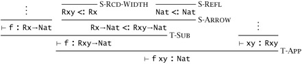
Here is another:

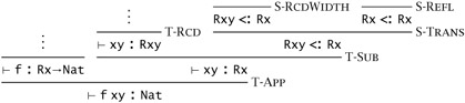
In fact, as the second example suggests, there are actually infinitely many typing derivations for any derivable statement in this calculus.

15.2.3 Solution

I count six: {a:Top,b:Top}, {b:Top,a:Top}, {a:Top}, {b:Top}, {}, and Top.

For example, let

   S₀ = {}   S₁ = {a:Top}   S₂ = {a:Top,b:Top}   S₂ = {a:Top,b:Top,c:Top}   etc.

For example, let T₀ = S₀→Top, T₁ = S₁→Top T₂ = S₂→Top, etc.

15.2.4 Solution

(1) No. If there were, it would have to be either an arrow or a record (it obviously can't be Top). But a record type would not be a subtype of any of the arrow types, and vice versa. (2) No again. If there were such an arrow type T₁→T₂, its domain type T₁ would have to be a subtype of every other type S₁; but we have just seen that this is not possible.

15.2.5 Solution

Adding this rule would not be a good idea if we want to keep the existing evaluation semantics. The new rule would allow us to derive, for example, that Nat × Bool <: Nat, which would mean that the stuck term (succ (5,true)) would be well typed, violating the progress theorem. The rule is safe in a "coercion semantics" (see §15.6), though even there it raises some algorithmic difficulties for subtype checking.

15.3.1 Solution

By adding bogus pairs to the subtype relation, we can break both preservation and progress. For example, adding the axiom

                          {x:{}} <: {x:Top→Top}

allows us to derive Г ⊢ t : Top, where t = ({x={}}.x){}. But t → {}{}, which is not typable-a violation of preservation. Alternatively, if we add the axiom

                               {} <: Top→Top

then the term {}{} is typable, but this term is stuck and not a value-a violation of progress.

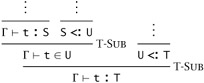
On the other hand, taking away pairs from the subtype relation is actually harmless. The only place where the typing relation is mentioned in the statement of the progress property is in the premises, so restricting the subtype relation, and hence the typing relation, can only make it easier for progress to hold. In the case of the preservation property, we might worry that taking away the transitivity rule, in particular, would cause trouble. The reason it does not is, intuitively, that its role in the system is actually inessential, in the sense that the subsumption rule T-SUB can be used to recover transitivity.

For example, instead of

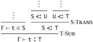
we can always write:

15.3.2 Solution

By induction on subtyping derivations. By inspection of the subtyping rules in Figures 15-1 and 15-3, it is clear that the final rule in the derivation of S <: T₁→T₂ must be S-REFL, S-TRANS, or S-ARROW.

If the final rule is S-REFL, then the result is immediate (since in this case S = T₁→T₂, and we can derive both T₁ <: T₁ and T₂ <: T₂ by reflexivity).

If the final rule is S-TRANS, then we have subderivations with conclusions S <: U and U <: T₁→T₂ for some type U. Applying the induction hypothesis to the second subderivation, we see that U has the form U₁→U₂, with T₁ <: U₁ and U₂ <: T₂. Now, since we know that U is an arrow type, we can apply the induction hypothesis to the first subderivation to obtain S = S₁→S₂ with U₁ <: S₁ and S₂ <: U₂. Finally, we can use S-TRANS twice to reassemble the facts we have established, obtaining T₁ <: S₁ (from T₁ <: U₁ and U₁ <: S₁) and S₂ <: T₂ (from S₂ <: U₂ and U₂ <: T₂).

If the final rule is S-ARROW, then S has the desired form and the immediate subderivations are exactly the facts we need about the parts of S.
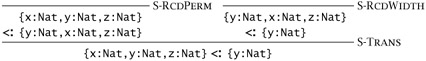
By induction on subtyping derivations. Again, inspecting the subtyping rules reveals that the final rule in the derivation of S <: {l_i :T_i ⁱÎ^l..n} must be S-REFL, S-TRANS, S-RCDWIDTH, S-RCDDEPTH, or S-RCDPERM. The case for S-REFL is trivial. The cases for S-RCDWIDTH, S-RCDDEPTH, and S-RCDPERM are all immediate.

If the final rule is S-TRANS, then we have subderivations with conclusions S <: U and U <: {l_i:T_i ⁱÎ^l..n} for some type U. Applying the induction hypothesis to the second subderivation, we see that U has the form {u_a:U_a ^aÎl..o}, with {l_i ^iÎl..n} ⊆ {u_a ^aÎl.,o} and with U_a <: T_i for each l_i = u_a. Now, since we know that U is a record type, we can apply the induction hypothesis to the first subderivation to obtain S = {k_j:S_j ^jÎl..m}, {u_a ^aÎl..o} ⊆ {k_j ^jÎl..m} and with S_j <: U_a for each u_a = k_j. Reassembling these facts, we obtain {l_i ^iÎl..n} ⊆ {k_j ^jÎl..m} by the transitivity of set inclusion, and S_j <: T_i by S-TRANS for each l_i = k_j, since each label in T must also be in U (i.e., l_i, must be equal to u_a for some a), and then we know S_j <: U_a and U_a <: T_i. (The awkward choice of metavariable names here is unavoidable: there just aren't enough roman letters to go around.)

15.3.6 Solution

Both parts proceed by induction on typing derivations. We show the argument just for the first part.

By inspection of the typing rules, it is clear that the final rule in a derivation of ⊢ v : T₁→T₂ must be either T-ABS or T-SUB. If it is T-ABS, then the desired result is immediate from the premise of the rule. So suppose the last rule is T-SUB.

From the premises of T-SUB, we have ⊢ v : S and S <: T₁→T₂. From the inversion lemma (15.3.2), we know that S has the form S₁→S₂. The result now follows from the induction hypothesis.

16.1.2 Solution

Part (1) is a straightforward induction on the structure of S.

For part (2), we first note that, by part (1), if there is any derivation of S <: T, then there is are reflexivity-free one. We now proceed by induction on the size of a reflexivity-free derivation of S <: T. Note that we are arguing by induction on the size of the derivation, rather than on its structure, as we have done in the past. This is necessary because, in the arrow and record cases, we apply the induction hypothesis to newly constructed derivations that do not appear as subderivations of the original.

If the final rule in the derivation is anything other than S-TRANS, then the result follows directly by the induction hypothesis (i.e., by the induction hypothesis, all of the subderivations of this final rule can be replaced by derivations not involving transitivity; since the final rule itself is not transitivity either, the whole derivation is now transitivity-free). So suppose the final rule is S-TRANS-i.e., that we are given subderivations with conclusions S <: U and U <: T, for some type U. We proceed by cases on the pair of final rules in both of these subderivations.

Case ANY/S-TOP:

 T = Top

If the right-hand derivation ends with S-Top, then the result is immediate, since S <: Top can be derived from S-TOP no matter what S is.

Case S-TOP/ANY:

 U = Top

If the left-hand subderivation ends with S-TOP, we first note that, by the induction hypothesis, we may suppose that the right-hand subderivation is transitivity-free. Now, inspecting the subtyping rules, we see that the final rule in this subderivation must be S-TOP (we have already eliminated reflexivity, and all the other rules demand that U be either an arrow or a record). The result then follows by S-TOP.

Case S-ARROW/S-ARROW:	S = S₁→S₂	U = U₁→U₂	T = T₁→T₂
	U₁ <: S₁	S₂ <: U₂
	T₁ <: U₁	U₂ <: T₂

Using S-TRANS, we can construct derivations of T₁ <: S₁ and S₂ <: T₂ from the given subderivations. Moreover, these new derivations are strictly smaller than the original derivation, so the induction hypothesis can be applied to obtain transitivity-free derivations of T₁ <: S₁ and S₂ <: T₂. Combining these with S-ARROW, we obtain a transitivity-free derivation of S₁→S₂ <: T₁→T₂.

Case S-RCD/S-RCD:

Similar.

Other cases:

The other combinations (S-ARROW/S-RCD and S-RCD/S-ARROW) are not possible, since they place incompatible constraints on the form of U.

16.1.3 Solution

If we add Bool, then the first part of Lemma 16.1.2 needs to be modified a little. It should now read, "S <: S can be derived for every type S without using S-REFL except at type Bool." Alternatively, we can add a rule

                             Bool <: Bool

to the definition of subtyping and then show that S-REFL can be dropped from the enriched system.

16.2.5 Solution

By induction on declarative typing derivations. Proceed by cases on the final rule in the derivation.

Case T-VAR:

t = x

Г (x) = T

Immediate, by TA-VAR.

Case T-ABS:

t = λx:T₁.t₂

Г, x:T₁ ⊢ t₂ : T₂

T = T₁→T₂

By the induction hypothesis, Г, , for some S₂ <: T₂. By TA-ABS, Г . By S-ARROW, T₁→S₂ <: T₁→T₂, as required.

Case T-APP:

t = t₁ t₂

Г ⊢ t₁ : T₁₁→T₁₂

Г ⊢ t₂ : T₁₁

T = T₁₂

By the induction hypothesis, for some S₁ <: T₁→T₁₂ and for some S₂ <: T₁₁. By the inversion lemma for the subtype relation (15.3.2), S₁ must have the form S₁₁→S₁₂, for some S₁₁ and S₁₂ with T₁₁ <: S₁₁ and S₁₂ <: T₁₂. By transitivity, S₂ <: S₁₁. By the completeness of algorithmic subtyping, . Now, by TA-APP, , which finishes this case (since we already have S₁₂ <: T₁₂).

Case T-RCD:	t = {l_i =t_i ^iÎl..n}	Г ⊢ t_i : T_i	for each i
	T = {l_i : T_i ^iÎl..n}

Straightforward.

Case T-PROJ:

t = t₁ . l_j

Г ⊢ t₁ : {l_i :T_i ^iÎl..n}

T = T_j

Similar to the application case.

Case T-SUB:

t : S

S <: T

By the induction hypothesis and transitivity of subtyping.

16.2.6 Solution

The term λx:{a:Nat}.x has both the types {a:Nat}→{a:Nat} and {a:Nat}→Top under the declarative rules. But without S-ARROW, these types are incomparable (and there is no type that lies beneath both of them).

16.3.2 Solution

We begin by giving a mutually recursive pair of algorithms that, we claim (and will show, below), calculate the join J and meet M, respectively, of a pair of types S and T. The second algorithm may also fail, signaling that S and T have no meet.

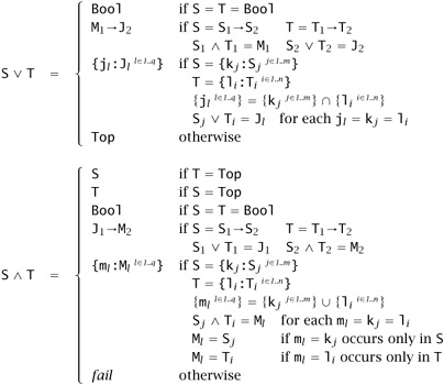
In the arrow case of the first algorithm, the call to the second algorithm may result in failure; in this case the first algorithm falls through to the last case and the result is Top. For example Bool→Top V {}→Top = Top.

It is easy to check that V and ∧ are total functions (i.e., never diverge): just note that the total size of S and T is always reduced in recursive calls. Also, the ∧ algorithm never fails when its inputs are bounded below:

< Free Open Study >