Pure Frontier Models

---

Consider the general composed error stochastic frontier estimation model given by

(1) 

where for j = 1, …,n

y_j is the dependent variable

x_j is a vector of measurements on independent variables in ℜ^m

θ is a vector of model parameters in ℜ^p

f(x_j,θ) is a "ceiling" type frontier model—that is, observations without other errors will fall beneath the level given by the ceiling model. A "floor" model is the opposite and the model specification becomes

(2) 

ε_j is a white noise error term with variance σ²

ω_j is a nonnegative inefficiency error for observation j, independent of the ε_j. Thus, a pure frontier (ceiling) model would be given by

(3) 

and similarly, a pure frontier (floor) model would appear as

(4) 

The ceiling model would be most appropriate if the behavior of the observations is such that "more is always better." That is, the observations represent attempts to maximize the dependent variable. Similarly, the floor model would be appropriate in the opposite case. From this point of view, the OLS model can sometimes be regarded as a "middle is better" situation. Figure 1 depicts a scattergram of data pairs with the ordinary least squares (OLS) regression model and a ceiling type frontier model.

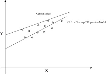
Figure 1: Ceiling versus OLS regression

It can be noted that the ceiling model is not necessarily the same as that obtained by raising the OLS model upwards until it just envelops the data points from above. This is, of course, a heuristic approach to estimating a ceiling model in two dimensions. A more dramatic difference can be seen for regression or frontier models that are specified to have zero-intercepts (so-called regression through the origin). Figure 2 depicts this contrast between an OLS and a floor frontier model for the same scattergram.

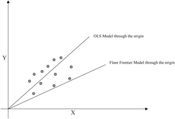
Figure 2: Models forced to pass through the origin

Figures 1 and 2 also suggest a motivation for the SFE models. Namely, the position and slope of the ceiling model depends heavily on just a few of the uppermost data pairs. On the possibility that those data pairs are unrepresentative outliers, then one has less confidence that the correct frontier model has been estimated. From the point of view of optimum seeking or purposeful behavior, such data points would represent unusually good performance in the nature of a lucky event. For the purposes of this research, we assume that any such data have been removed or adjusted appropriately. One might consider SFE models as motivated by a desire to smooth out the upper or lower boundaries with white noise adjustments as a more mechanical approach to this issue, however.

Various approaches to estimating such pure frontier models have been proposed. For example, if the sum of squares of the ω_j is minimized as the model fitting criterion, then that procedure is a maximum likelihood estimation (MLE) procedure when the ω_j are distributed as half-normal. Similarly, minimizing the sum of the ω_j is MLE when they are distributed with the exponential probability density function. In this work, we propose the latter criterion. Namely, we assume in the rest of this chapter that models of the type (3) and (4) will be fitted or estimated by the criterion of minimum Σ_jω_j, but we use a different, more general rationale than the above kinds of distribution assumptions to be explained below.

There are three reasons for this choice of criterion. First is the rationale of purposeful behavior. If each observation is interpreted as an attempt to reach the target or goal given by the frontier model, then the ωj may be regarded as distances from the target. As each attempt seeks to minimize such a distance, then over all instances or observations the sum of these would be minimized. That is, the criterion of minimum Σ_jω_j is taken as modeling purposeful behavior over repetitions of a single unit or over a set of units. This has been formalized in Troutt et al. (2000) as the maximum performance efficiency (MPE) estimation principle.

The second reason is that computation of a model solution for this criterion is flexible and straightforward. Typically, the model is a simple linear programming model easily solved with a spreadsheet solver. The model used in Troutt, Gribbin, Shanker and Zhang (2000) is an example.

The third reason is that a model aptness test is available for this criterion. Called the normal-like-or-better (NLOB) criterion, it consists of examining the fitted ω_j values. If these have a density sufficiently concentrated on the mode at zero, then the performance can be said to be as good or better than a bivariate normal model for a target such as a bull's-eye in throwing darts. Note that sometimes throwing darts is used as a metaphor for completely random guessing. Here we use it differently, however. If a data scattergram for dart hits is modeled well by a univariate density as steep or steeper than the normal, and with mode coincident to the target, then we regard this as very good performance, allowing for natural efficiency variation. The NLOB criterion can, in principle, be used with any distributional form for the fitted ω_j values. However, it appears most naturally suited to the case when these are gamma distributed. Complete details on applying the NLOB criterion may be found in Troutt et al. (2000).

---