Markov Chain Monte Carlo Techniques

---

Markov chain Monte Carlo (MCMC) methodology provides enormous scope for realistic statistical modelling and has become popular recently for Bayesian computation in complex statistical models. MCMC is essentially Monte Carlo integration using Markov chains. Bayesian analysis requires integration over possibly high-dimensional probability distributions to make inferences about model parameters or to make predictions. However, in the past, Bayesian inference has been hampered by the problem of evaluating the summaries of the posterior marginal densities by numerical integration. This problem becomes more acute when Bayesian statisticians have to solve high dimensional integrals. Complex numerical integration methods such as the Gaussian quadrature and Laplace approximation (Shun & McCullagh, 1995; Tierney & Kadane, 1986) are utilized. Monte Carlo integration draws samples from the required distribution and then forms sample averages to approximate expectations. The MCMC approach draws these samples by running a suitably constructed Markov chain for a long time. There are many ways of constructing these chains, but most of them, including the Gibbs sampler (Geman & Geman, 1984), are special cases of the general framework of Metropolis, Rosenbluth, Rosenbluth, Teller, & Teller (1953) and Hastings (1970). Many MCMC algorithms are hybrids or generalizations of the simplest methods: the Gibbs sampler and the Metropolis-Hastings algorithm. One may refer to the two mongraphs by Gilks, Richardson, & Spiegelhalter (1996) and Gamerman (1997) for more detail about Markov chain Monte Carlo method.

The Metropolis-Hastings Algorithm

Constructing such a Markov chain is not difficult. We first describe the Metropolis-Hastings algorithm. This algorithm is due to Hastings (1970), which is a generalization of the method first proposed by Metropolis et al. (1953).

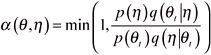
Let p(θ) be the distribution of interest. Suppose at time t, θ_t+1 is chosen by first sampling a candidate point η from a proposal density q(.| θ_t). The candidate η is accepted with probability If the candidate point is accepted, the next state becomes θ_t+1= η. If it is rejected, then θ_t+1= θ_t and the chain does not move. The proposed distribution is arbitrary and provided the chain is irreducible and aperiodic, the equilibrium distribution of the chain will be p(θ).

The Gibbs Sampler

Many statistical applications of MCMC have used the Gibbs sampler, which is easy to implement. Gelfand and Smith (1990) gave an overview, and suggested the approach for Bayesian computation. First, probability densities of an unknown parameter θ of interest are denoted as p(θ) = F'(θ), where F(θ) is the cumulative distribution function (CDF) of θ. Therefore, in the sequel, joint, conditional and marginal densities appear as p(θ, η), p(θ| η), and p(η). Now the Gibbs sampling algorithm is best described as follows:

1. Let θ = (θ₁, θ₂, ..., θ_k) be a collection of random variables.

2. Given arbitrary initial values θ₁ ⁽⁰⁾,...,θ_k ⁽⁰⁾ we draw θ₁ ⁽¹⁾ from the conditional distribution p(θ₁ | θ₂ ⁽⁰⁾,...,θ_k ⁽⁰⁾).

3. Then θ₂ ⁽¹⁾ from p(θ₂ | θ₁ ⁽¹⁾, θ₃ ⁽¹⁾...,θ_k ⁽⁰⁾) and so on up to θ_k ⁽¹⁾ θ_k ⁽¹⁾from p(θ_k | θ₁ ⁽¹⁾, θ₁ ⁽¹⁾...,θ_k-1 ⁽⁰⁾) to complete one iteration of the scheme.

This scheme is a Markov chain, with equilibrium distribution p(θ). After t such iterations we would arrive at (θ₁ ^(t), θ₂ ^(t), ...,θ_k ^(t) ) . Thus, for t large enough, θ^(t) can be viewed as a simulated observation from p(θ). Provided we allow a suitable burn-in time, θ^(t), θ^(t+1), θ^(t+2),... can be thought of as a dependent sample from p(θ).

Similarly, suppose we wish to estimate the marginal distribution of a variable η which is a function g(θ₁, θ₂, K, θ_k) of θ. Evaluating g at each of the θ^(t) provides a sample of η. Marginal moments or tail areas are estimated by the corresponding sample quantities. Densities may be estimated using kernel density estimates (Devroye, 1987; Silverman, 1986).

Sampling Methods Used With the Gibbs Sampler

The Gibbs sampler involves sampling from full conditional distributions. It is essential that sampling from full conditional distributions is highly efficient computationally. Rejection sampling is a possible technique for sampling independently from a general density p(q) where p(θ) is intractable analytically.

Rejection sampling requires an envelope function g of p(θ) where g(θ) ≥ p(θ) for all θ. Samples are drawn from a density proportional to g, and a sampled point p(θ) is accepted with probability g(θ)/p(θ).

The adaptive rejection sampling (ARS) method was proposed by Gilks and Wild (1992). In the general rejection sampling method, finding a tight envelope functiong g is difficult. However in many applications of Gibbs sampling, the full conditional densities p(θ) are often log-concave

Gilks and Wild (1992) proposed the adaptive rejection sampling method to sample from a complicated full conditional density which satisfies the log-concavity condition. They showed that an envelope function for log p(θ) can be constructed by drawing tangents to log p at each abscissae for a given set of abscissae. An envelope between any two adjacent abscissae is then constructed from the tangents at either end of that interval. Secants are drawn through log p(θ) at adjacent abscissae. The envelope is piece-wise exponential for which sampling is straightforward. We will use the adaptive rejection sampling method for sampling from conditional densities. One may refer to the article by Gilks and Wild (1992) for more theoretical details about their method.

---