The Fourier Transform

As mentioned in the introduction to this chapter, there are two ways in which you can characterize a signal. The first way is in the time domain where the signal amplitude is expressed as a function of time, as in Eq. (22.1).

Equation 22.1

The signal can also be characterized in the frequency domain by expressing the frequency amplitude as a function of frequency, as in Eq. (22.2).

Equation 22.2

The frequency, f , in Eq. (22.2) is in units of 1/sec or Hz and is equal to 1/ T , where T is the period of the function. The frequency domain is sometimes characterized using, w = 2 p f , the angular frequency in units of radians/sec.

The Fourier transform is used to switch back and forth between the time and frequency domains. It is based on the Fourier series that allows you to express any periodic function, g ( t ), as an infinite series of sinusoidal functions.

Equation 22.3

The w _n term in Eq. (22.3) is given by the expression w _n = 2 p nf . The signal energy at a given frequency, f _n , is equal to the sum of the square of the a and b coefficients, ). Determining the energy spectrum of a signal is an important use of Fourier transforms.

The Fourier series can be also expressed in complex form.

Equation 22.4

The variables on the right-hand side of Eq. (22.4) are defined in Eq. (22.5).

Equation 22.5

The continuous or integral Fourier transform is based on Eq. (22.4). It relates the characterization of a signal in the frequency domain to its characterization in time domain.

Equation 22.6

The inverse Fourier transform, going from frequency to time domains, is given by a similar expression.

Equation 22.7

The reason to define both forward and inverse transforms is to provide the ability to switch back and forth between the time and frequency domains. The inverse transform of the forward transform of a function should return the original function. The only differences between Eq. (22.6) and Eq. (22.7) are the change of sign in the exponential power term and the different function and variable of integration. The time-frequency domains are not the only ones to which Eq. (22.6) and Eq. (22.7) can be applied. They could be used, for instance, to switch between the position and inverse wavelength domains.

Table 22.1. Time and Frequency Function Relationships

X(T)	X(F)
Real and even	Real and even
Real and odd	Imaginary and odd
Imaginary and even	Imaginary and even
Imaginary and odd	Real and odd

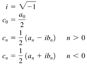
One reason to use the complex form of the Fourier series is that the time and frequency equations may be complex, containing both real and imaginary parts . Even if the original signal is completely real, the frequency response obtained from the Fourier transform may have both real and imaginary components . The characteristics of the frequency response depend on whether the function is real or imaginary and whether the function is even or odd. An odd function, such as the sine function, is one where g ( t ) = “ g ( “ t ). An even function, such as the cosine function, is one where g ( t ) = g ( “ t ). Table 22.1 summarizes some of the relationships between the two domains.

One thing to notice about Table 22.1 is that when you transform a sine wave, which is a real, odd function, the resulting frequency response is in the imaginary plane.

What we have discussed in this section and will cover in the rest of this chapter is a 1-D Fourier transform that is used to travel between time and frequency domains. This type of transform is typically applied to electronic or acoustic signal analysis. There are also multidimensional Fourier transforms that are used for optical or image analysis applications. We won't discuss multidimensional Fourier transforms in this book. For more information on them, consult an appropriate Fourier transform reference.