Applying Basic Formatting

You can use a variety of formatting options to emphasize parts of a worksheet and display data in different ways. Here you ll use some of the common formatting options available on the Formatting toolbar and some less common ones available in the Format Cells dialog box. You ll also learn a quick way to adjust column widths.

Changing the Look of Characters

When you want to make tables of data easier to read, you can use character formatting to distinguish different categories of information. For example, you can use a different font or style to make certain elements stand out. Try this:

1. Select A1:D1, the range that contains the headings.

2. On the Formatting toolbar, click the Bold button, and then change the font size to 12 .

   You might need to use the toolbar s move handle or click the Toolbar Options button to display the Bold button. The headings are now displayed larger and in bold.

Changing Alignment

As you know, Excel left-aligns text and right-aligns values by default. You can override the default alignment by using the alignment buttons . Here s how:

1. With A1:D1 still selected, click first the Align Left button and then the Align Right button on the Formatting toolbar, noting the effects.

2. Click the Center button to center all the entries in the column, which is a typical way to display headings.

Grouping and Ungrouping Worksheets

When you want to add the same information or the same type of formatting across more than one worksheet, you can group the worksheets. Then changes you make to the active worksheet are reflected in all the other worksheets in the group. To group worksheets, activate the first sheet you want included in the group, hold down the Shift key, and click the tabs of each of the other worksheets you want included in the group. Make whatever entries or formatting changes you want applied to the group. Then to ungroup worksheets, hold down the Shift key and click the first sheet in the group to deselect the others.

 

Formatting Entries

Earlier, you entered dates in column B in a variety of formats. The entries in column A aren t aligned because Excel is treating some of them as text and some as numbers . In this section, we ll use the Format Cells dialog box to apply a consistent format to these entries, as well as to better present the invoice amounts in column D. Follow these steps:

1. Select B2:B13, which contain the dates, and then click Cells on the Format menu.

   Excel displays the Format Cells dialog box, shown here, from which you can make many formatting changes:

   

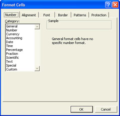
2. On the Number tab, select Date in the Category list, select 3/14/02 (or its equivalent) in the Type list, and click OK .

3. Select A2:A13, and click Cells on the Format menu

4. In the Category list on the Number tab, select the Text category, and then click OK .

   You can also tell Excel to treat an individual entry as text by typing an apostrophe at the beginning of the entry.

   Now let s format the entries in column D as currency, using a different method to access the Format Cells dialog box.

5. Select D2:D13, right-click the selection, and then click Format Cells on the shortcut menu.

6. In the Format Cells dialog box, click Currency in the Category list on the Number tab, and accept the default settings by clicking OK .

   Excel automatically adjusts the width of the column to accommodate the new formatting.

AutoFormats

An autoformat is a predefined combination of formatting for use with certain kinds of worksheets. Although the autoformats that come with Excel don t work well unless you set up your worksheet with them in mind, using autoformats is a great way to become familiar with the many effects you can create with combinations of fonts, lines, colors, and shading to produce fancylooking reports with the click of a button. To apply an autoformat, first select the range of cells you want to format, and then click AutoFormat on the Format menu. When the AutoFormat dialog box appears, select an option from the list, and click OK. If you don t find a format that produces the exact look you want, you can make refinements using the Font, Fill Color, Font Color , and Borders buttons on the Formatting toolbar or the options available in the Format Cells dialog box. You can also customize an autoformat by clicking the Options button in the AutoFormat dialog box and selecting or deselecting the options in the Formats to Apply area. If you decide not to use a worksheet autoformat after all, select the formatted range, click AutoFormat on the Format menu, select None in the list, and then click OK.

 

Adjusting the Width of a Column

As a finishing touch for this worksheet, let s adjust the widths of columns A, B, and D so that all the headings are visible and fit neatly in their cells:

1. Move the mouse pointer to the dividing line between the headers of columns A and B .

   The pointer changes to a vertical bar with two opposing arrows.

2. Hold down the left mouse button and then drag to the right until column A is wide enough to display the Job Number heading.

   As you drag, the width is displayed in a box above the pointer.

3. Release the mouse button when you think that the heading will fit.

4. To change the width of column B, move the mouse pointer to the dividing line between columns B and C, and then double-click.

   The column width automatically adjusts to the width of the widest cell in the column. You can also select the column and click Column and then AutoFit Selection on the Format menu.

   Now let s try a different method to widen column D.

5. Select D1 , and click Column and then Width on the Format menu.

   Excel displays the Column Width dialog box shown here:

   

6. Type 20 , and press Enter .

   The results are shown in this graphic:

   

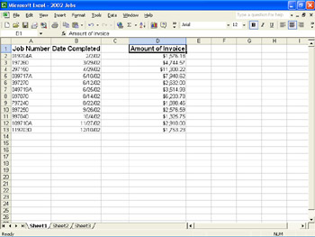
7. Save the workbook.

   You can adjust the height of rows the same way you adjust the width of columns. Simply drag the bottom border of the row header up or down, or click Row and then Height on the Format menu to make the row shorter or taller.

Changing the standard width

To change Excel s standard column width of 8.43 characters, click Column and then Standard Width on the Format menu, type a new value in the Standard Width dialog box, and click OK. (Any columns whose widths you have set manually retain their custom widths, but all the other columns adopt the new standard width.)